32, 64, 128 but could also be 100from random import shuffle
training = list(range(1,11)) # each index points to a training sample, could be a matrix x=HxWx3, label y
shuffle(training)
converge, it, max_it, k, epoch = False, 0, 100, 3, 0
while not converge and it < max_it: # you training convergence scheme
print(f'[Epoch {epoch}]')
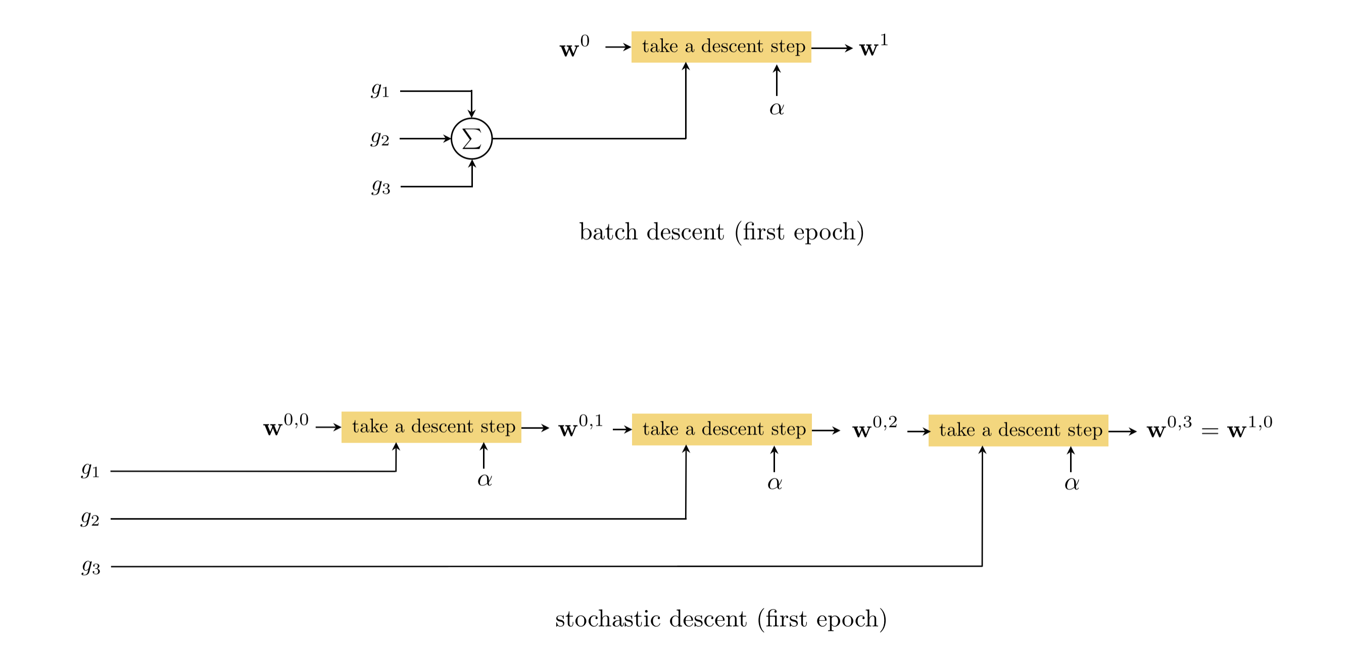
for b in range(0, len(training), k): # Data Loader gives you a batch k x matrices
mini_batch = training[b:b+k] # so mini-batch is a tensor HxWx3xk
if len(mini_batch) != k: # a possible way of handling the offset
continue
print('SGD step taken over', mini_batch) # compute the loss/gradients and upate your model
loss.backward() # get the gradients
optimizer.step() # incorporate in the model
# check convergence and set it to True
it += 1
epoch += 1 # an epoch is done, we reshuffle the training set
shuffle(training)
> Original unshuffled training set [1, 2, 3, 4, 5, 6, 7, 8, 9, 10]
> Training set [10, 8, 1, 2, 6, 4, 9, 7, 5, 3]
[Epoch 0]
SGD step taken over [10, 8, 1]
SGD step taken over [2, 6, 4]
SGD step taken over [9, 7, 5]
> Training set [1, 10, 6, 9, 3, 7, 8, 4, 5, 2]
[Epoch 1]
SGD step taken over [1, 10, 6]
SGD step taken over [9, 3, 7]
SGD step taken over [8, 4, 5]
> Training set [6, 3, 10, 5, 9, 8, 4, 7, 2, 1]
[Epoch 2]
SGD step taken over [6, 3, 10]
SGD step taken over [5, 9, 8]
SGD step taken over [4, 7, 2]
> Training set [1, 2, 5, 10, 6, 7, 9, 8, 3, 4]
[Epoch 3]
SGD step taken over [1, 2, 5]
SGD step taken over [10, 6, 7]
SGD step taken over [9, 8, 3]
> Training set [2, 3, 1, 9, 6, 8, 4, 10, 7, 5]
[Epoch 4]
With NN random initialization from a distribution (There are different methods). We do not set them all to zero
Below this holds for the final linear layer: $$ \underbrace{\mbf{Y}}_{\mathbb{R}^{Kxn}} = \underbrace{\mbf{W}}_{\mathbb{R}^{K\times d}}\underbrace{\mbf{X}_b}_{\mathbb{R}^{d\times n}} + \underbrace{\mbf{b}}_{\mathbb{R}^K}$$
Loss in NN in non-convex with lots of local-minima so stochasticity adds noise that let the optimization escape from local minima.
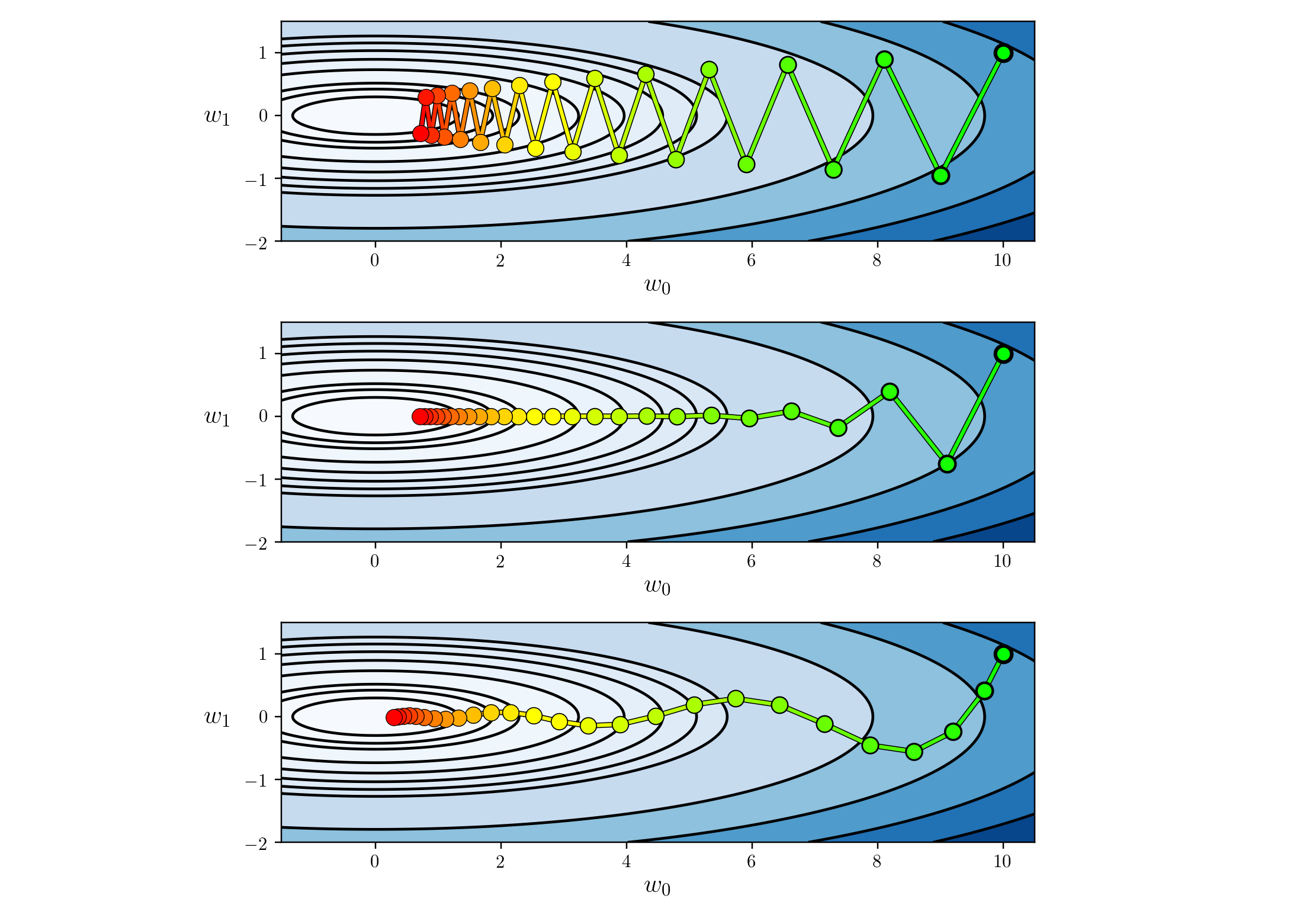
Top: SGD: Bottom: SGD with momentum increasing memory of previous steps
$$\bmf{\theta} \leftarrow \bmf{\theta} - \gamma \bmf{\Delta}_{t}$$
Repeat until convergence:
$$\bmf{\theta} \leftarrow \bmf{\theta} - \gamma \bmf{\Delta}_{t+1}$$
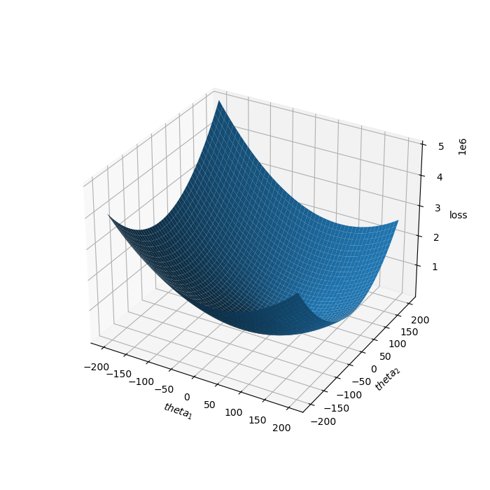
If you increase the dimensionality of the input data $\mbf{x}$ and thus also those of the parameters $\bmf{\theta}$ we can't draw the loss surface anymore but loss still remains convex, which means that there is a single global optimum.
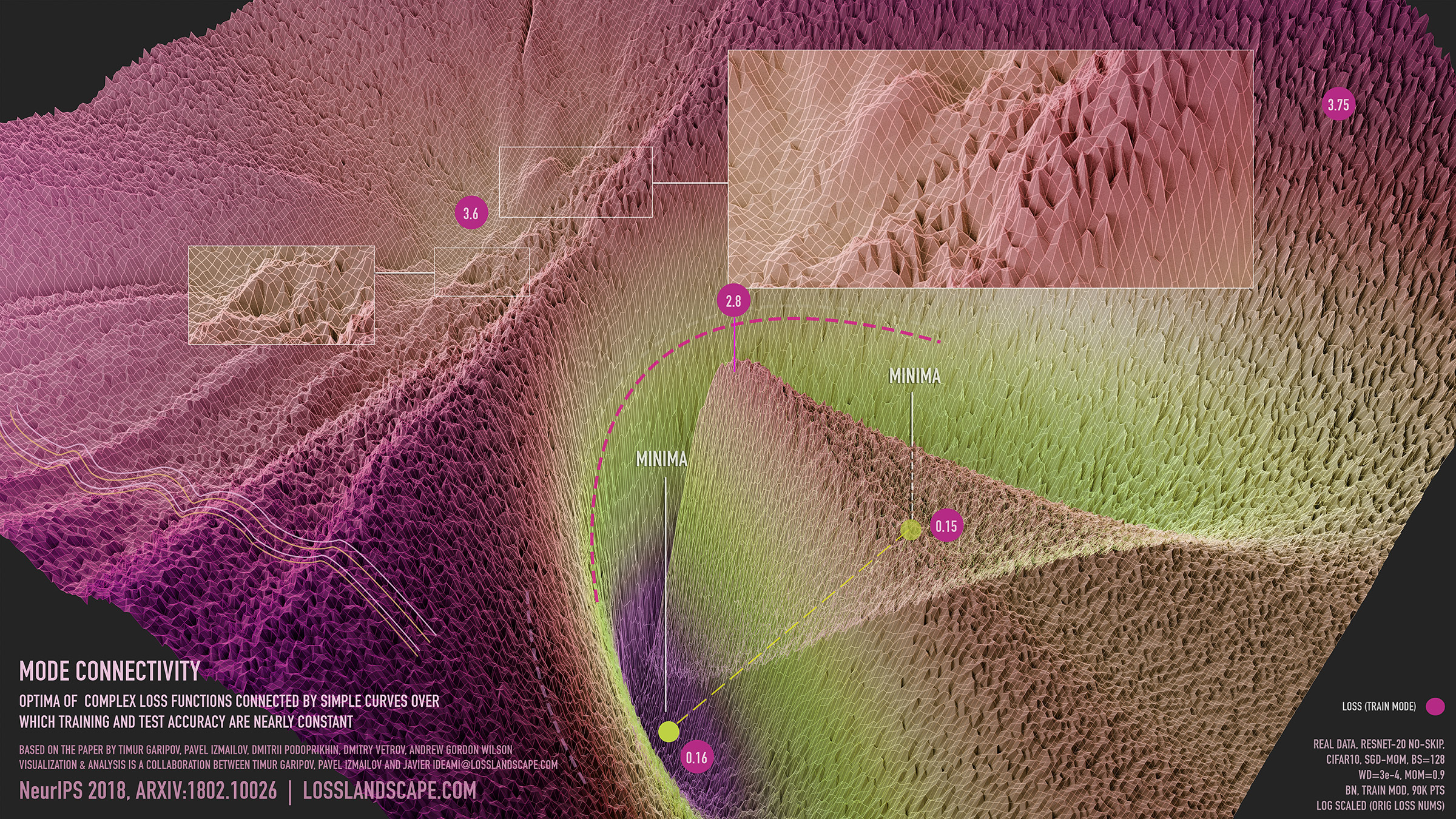
Visualization of mode connectivity for ResNet-20 with no skip connections on ImageNet dataset. The visualization by Javier Ideami

Noisy moons: This is logistic regression on noisy moons dataset from sklearn which shows the smoothing effects of momentum based techniques (which also results in over shooting and correction). The error surface is visualized as an average over the whole dataset empirically, but the trajectories show the dynamics of minibatches on noisy data. The bottom chart is an accuracy plot.

Long valley: Algos without scaling based on gradient information really struggle to break symmetry here - SGD gets no where and Nesterov Accelerated Gradient / Momentum exhibits oscillations until they build up velocity in the optimization direction. Algos that scale step size based on the gradient quickly break symmetry and begin descent.

Yikes! $12\times 10^9$ floating points parameters to train
DALL·E is a 12-billion parameter version of GPT-3 trained to generate images from text descriptions, using a dataset of text–image pairs. We’ve found that it has a diverse set of capabilities, including creating anthropomorphized versions of animals and objects, combining unrelated concepts in plausible ways, rendering text, and applying transformations to existing images.
You will meet them at Deep Learning course
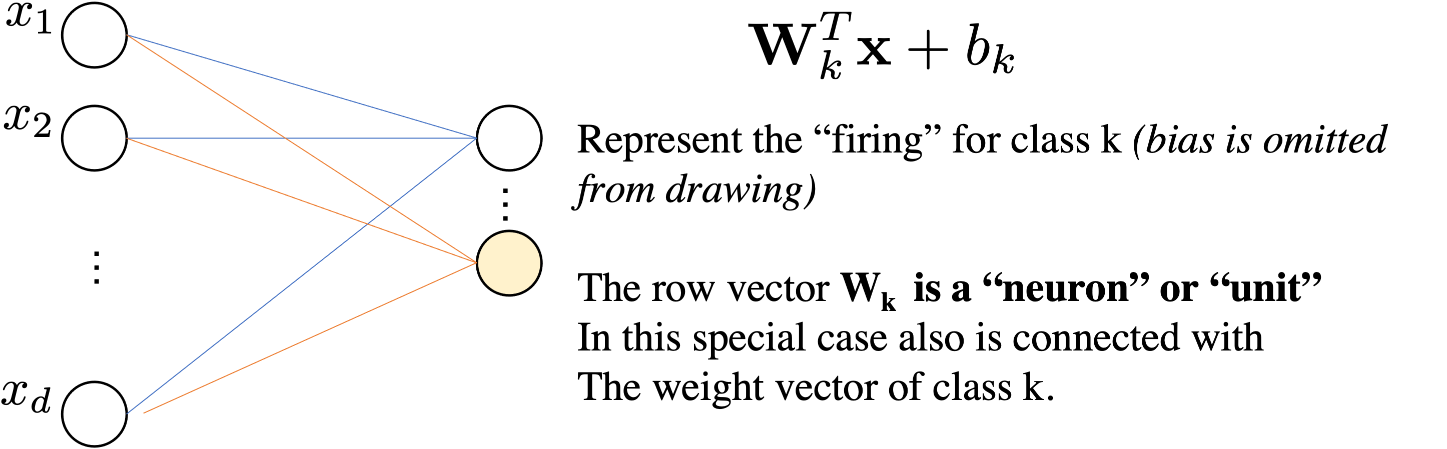
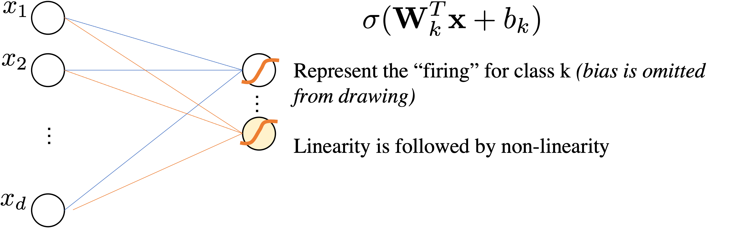
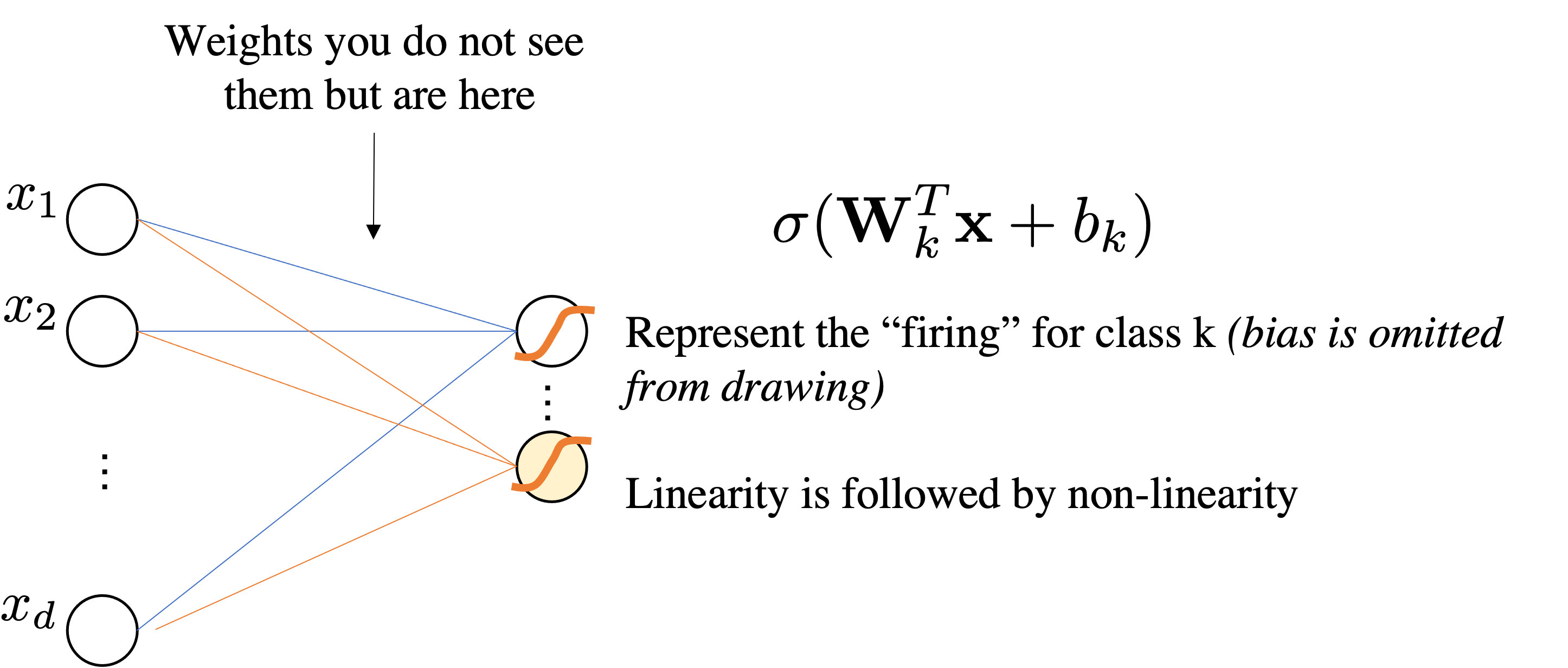
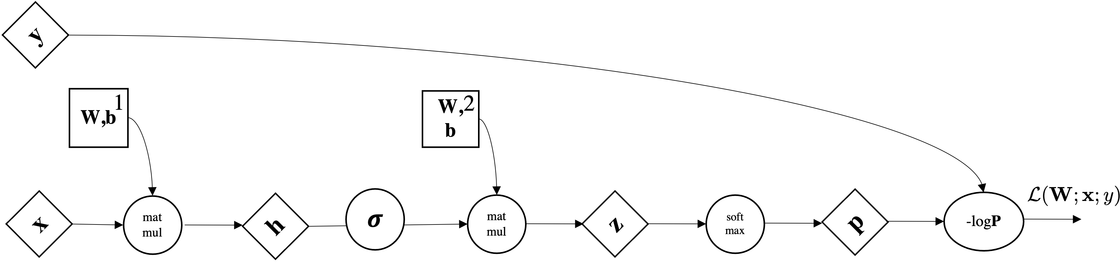
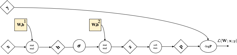
Let's consider our linear softmax regressor
$$ \underbrace{\mbf{z}}_{\mathbb{R}^{Kx1}} = \underbrace{\mbf{W}}_{\mathbb{R}^{K\times d}}\underbrace{\mbf{x}}_{\mathbb{R}^{d\times1}} + \underbrace{\mbf{b}}_{\mathbb{R}^K}$$We interpret as Linear Layer $\mathbf{W} \mathbf{x}+\bmf{b}$ followed by Non-Linear Activation function $\sigma$
$$ \sigma(\mathbf{W} \mathbf{x} + \bmf{b})=\sigma \circ\left(\begin{array}{cccc} w_{11} & w_{12} & \cdots & w_{1 d} \\ w_{21} & w_{22} & \cdots & w_{2 d} \\ \vdots & \cdots & \ddots & \vdots \\ w_{k 1} & w_{m 2} & \cdots & w_{k d} \end{array}\right)\left(\begin{array}{c} x_{1} \\ x_{2} \\ \vdots \\ x_{d} \end{array}\right)+ \left(\begin{array}{c} b_{1} \\ b_{2} \\ \vdots \\ b_{k} \end{array}\right) =\sigma \circ\left(\begin{array}{c} z_{1} \\ z_{2} \\ \vdots \\ z_{k} \end{array}\right) $$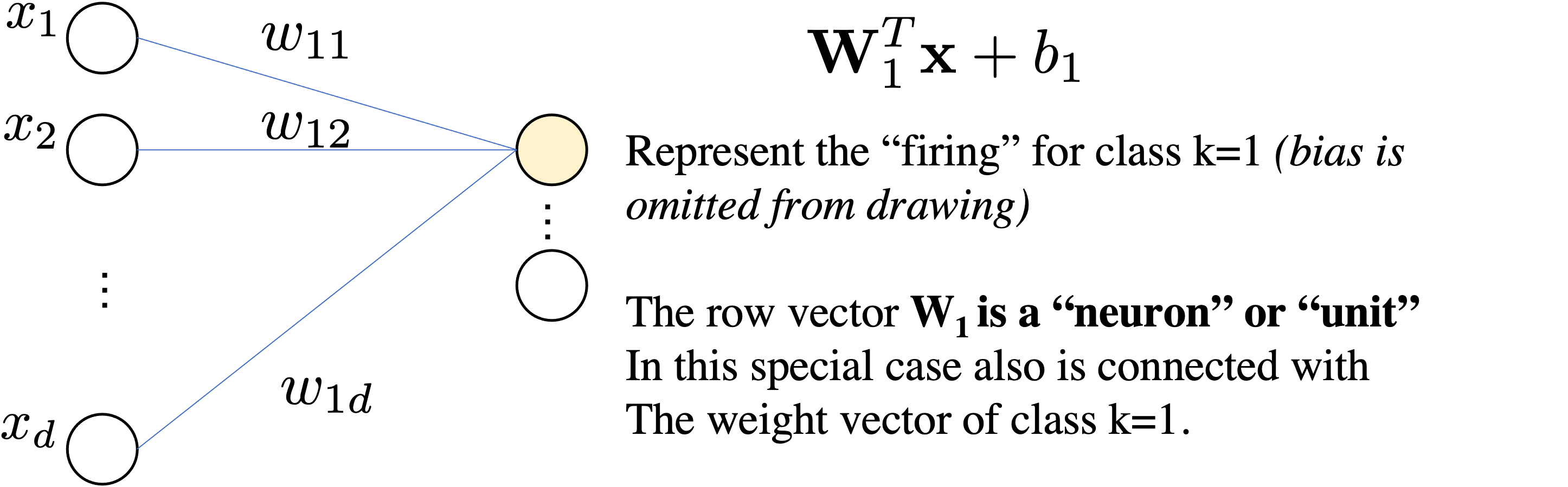
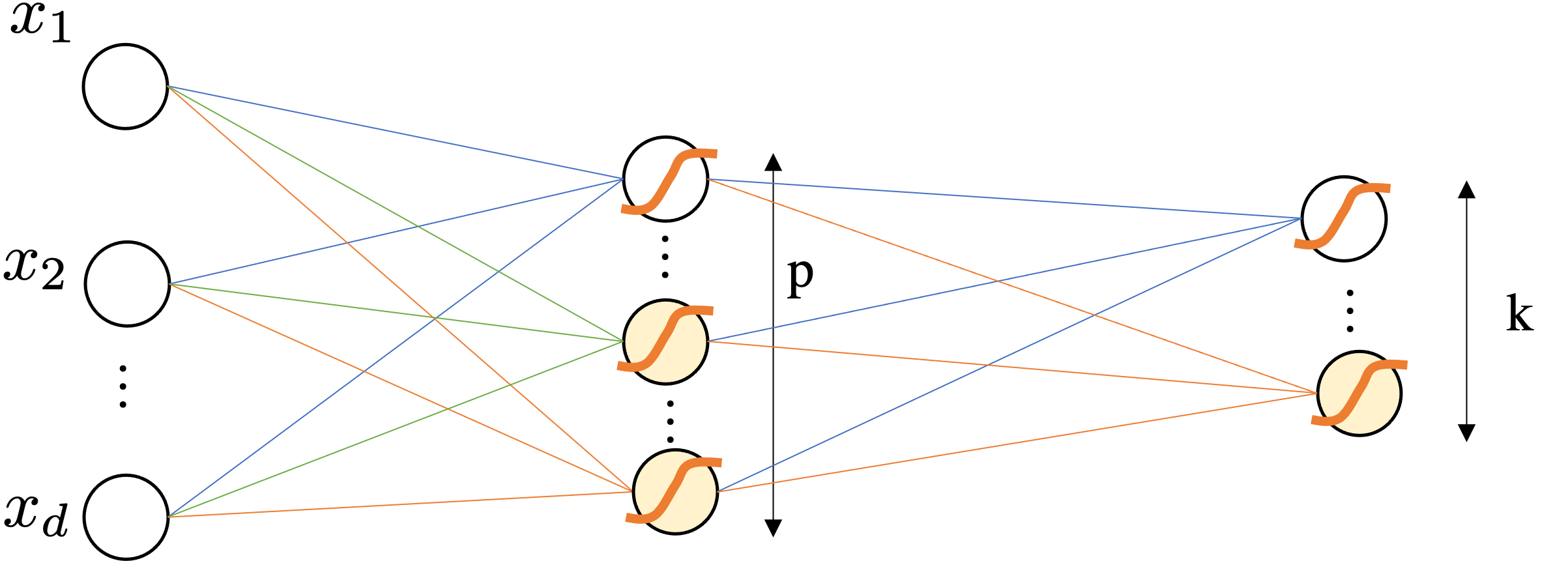
Because it maps the original attribute in $d$ from an dimensionality $p$ and then $p$ is used for classifying.
A priori you do not know what $\mathbf{W}^1$ may learn.
$$\mbf{p}=\sigma(\mathbf{W}^2\underbrace{\left(\sigma(\mathbf{W}^1 \mathbf{x} + \bmf{b}^1) \right)}_{\bmf{\phi}(x)} + \bmf{b}^2)$$$$\text{dim. analysis:} \quad d \mapsto p \mapsto k$$Very important: Activation Functions are computed element-wise.
$$ \sigma(z)= \frac{1}{1+\exp^{-z}} \quad \text{sigmoid or logistic function}$$Very important: Activation Functions are computed element-wise.
$$ \sigma(z)= \frac{1}{1+\exp^{-z}} \quad \text{sigmoid or logistic function}$$

Very important: Activation Functions are computed element-wise.
$$ \sigma(z)= \max(0,z) \quad \text{ReLu}$$

How many trainable parameters do you have with a MLP with input features in $\mathbb{R}^d$, a first layer with $p$ units/neurons and another layer with $k$ units/neurons that model the $k$ classes for classification. Assume all layers have the bias term.
We have two layers:
Total params = $(d \times p + p ) +(p \times k + k )$
so if $d=100$, $p=2000$, and $k=10$. Total params = 222,010
2 layers
3 layers
Consider $\sigma$ as Sigmoid activation function everywhere, what happens if $\mbf{W}$ are zeros?
No matter what is the input, the output will be always $\sigma(0)=0.5$, in other words a constant vector.
$$ \begin{aligned} &\mbf{z}^{[1]}=\mbf{W}^{[1]} \mbf{x}^{(i)}+\mbf{b}^{[1]} \\ &\mbf{a}^{[1]}=\sigma\left(\mbf{z}^{[1]}\right) \\ &\mbf{z}^{[2]}=\mbf{W}^{[2]} \mbf{a}^{[1]}+\mbf{b}^{[2]} \\ &\mbf{a}^{[2]}=\sigma\left(\mbf{z}^{[2]}\right) \\ &\mbf{z}^{[3]}=\mbf{W}^{[3]} \mbf{a}^{[2]}+\mbf{b}^{[3]} \\ &\hat{y}^{(i)}=\mbf{a}^{[3]}=\sigma\left(\mbf{z}^{[3]}\right) \end{aligned} $$NO, it won't!
Each element of the activation vector will be a scaled version of the input. This behavior will occur at all layers of the neural network. As a result, when we compute the gradient, all neurons in a layer will be equally responsible for anything contributed to the final loss. We call this property symmetry.
This means each neuron (within a layer) will receive the exact same gradient update value (i.e., all neurons will learn the same thing).
Randomness breaks the symmetric so that each neuron learns different things (gradients updates are different).
$$\mbf{W}_{ij} \sim \mathcal{U}(-0.1,0.1)$$$$\mbf{W}_{ij} \sim \mathcal{N}(0,0.01)$$Idea: For a single layer, consider the variance of the input to the layer as $\sigma^{in}$ and the variance of the output (i.e., activations) of a layer to be $\sigma^{out}$. Xavier/He initialization encourages $\sigma^{in}$ to be similar to $\sigma^{out}$.
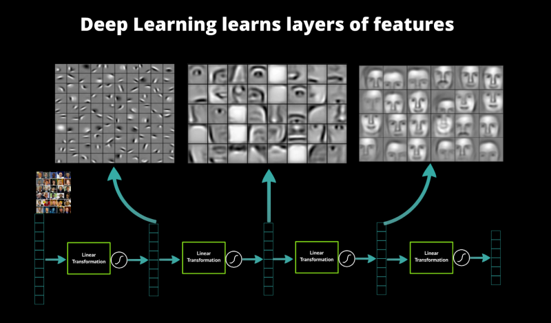
In principle, we can compose how many layers we want.
Think of each layer has learning a feature map on top of the previous feature map and then you have your final layer for your task at hand (classification, regression)
$$ \mathbf{y}=f \circ(\sigma \circ f) \circ \cdots \circ(\sigma \circ f)(\mathbf{x}) $$Given a continuous function $\mbf{y}=f(\mbf{x})$ where $\mbf{x} \in \mathbb{R}^d$ and $\mbf{y} \in \mathbb{R}^k$, considering only a bounded region of $\mbf{x}$, there exists a single-hidden-layer $NN_\theta$ with a finite number of neurons/units in the hidden layer, such that:
$$\vert f(\mbf{x}) - NN_\theta(\mbf{x}) \vert \le \epsilon $$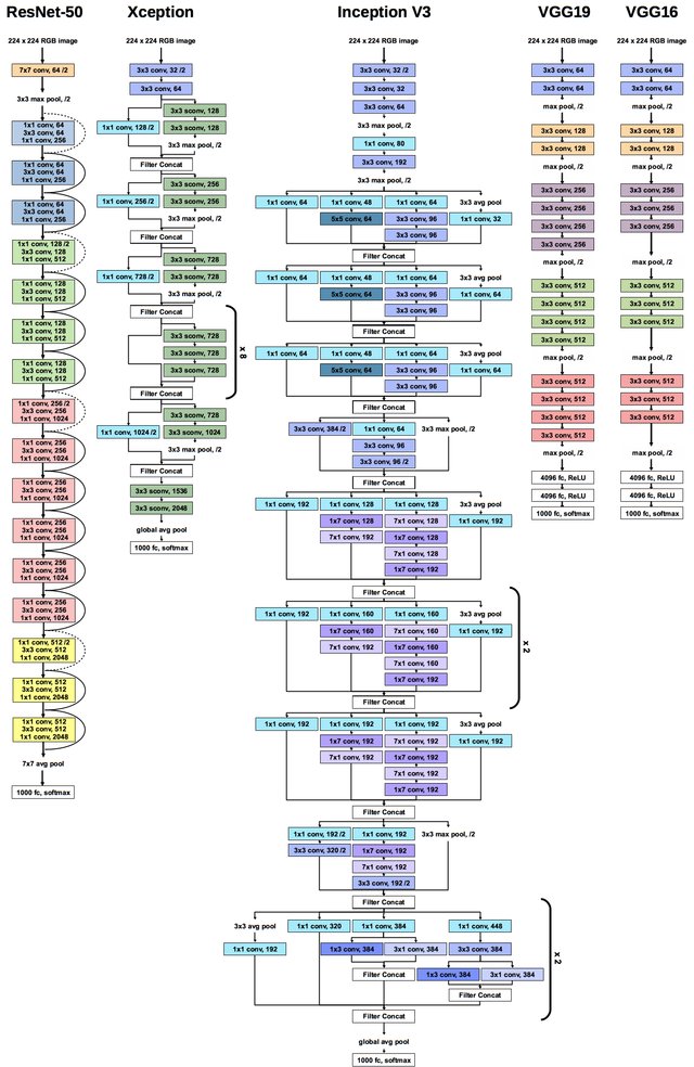
Implement the definition of derivative and apply it numerically on vectors:
$$\frac{df}{dx}(x) = \lim_{\epsilon \rightarrow 0}\frac{f(x+\epsilon) - f(x)}{\epsilon}.$$How do we read this formula for finite difference with neural net?
Assume $\mathbf{W}$ is your matrix and $w=\mathbf{W}_{ij}$ is a scalar inside your matrix.
For i,j=1....dims:
L(w)L(w+eps)[L(w+eps)-L(w)]/eps at position ij, so store it in $\nabla_{\mbf{W}}\mathcal{L}_{ij}$At the end you have your numerical gradients $\nabla_{\mbf{W}}\mathcal{L}_{ij}$.
https://people.idsia.ch/~juergen/who-invented-backpropagation.html
$\forall l \in [1\ldots,L]$:
$\forall l \in [1\ldots,L]$:
Returning to functions of a single variable, suppose that $y = f(g(x))$ and that the underlying functions $y=f(u)$ and $u=g(x)$ are both differentiable. The chain rule states that
$$\frac{dy}{dx} = \frac{dy}{du} \frac{du}{dx}.$$What is the derivative of loss wrt $x$ in the equation below? $$y = loss\big(g(h(i(x)))\big)$$
In pytorch this mechanism is called autograd
Can be viewed as a function of:
import torch
import random
random.seed(0) # to fix the random seed to make the code deterministic
torch.manual_seed(0) # to fix the random seed to make the code deterministic
print(torch.__version__)
2.1.2
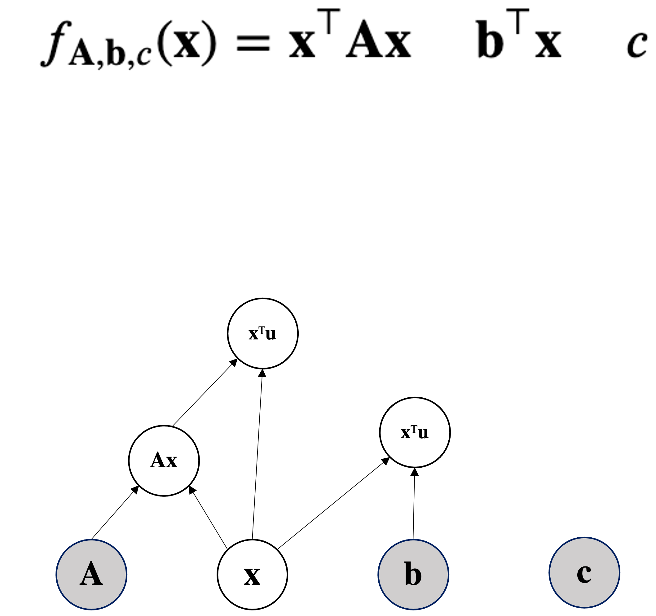
We assume the parameters $\mbf{\theta}$ as given and fix and we optimize the input $\mbf{x}$.
We assume $\mbf{x} \in \mathbb{R}^2$.
## params
A = torch.tensor([[0., 2.], [2.,0.]]) # 2x2
b = torch.tensor([[-0.5],[ 0.5]])  # 2x1
c = torch.tensor([-2.], dtype=torch.float32) # 1x1
## input
x = torch.tensor([1., 1.], requires_grad=True) # 1x  Note how here we require the gradients
thetas = (A, b, c) # pack the parameters
A.shape, b.shape, c.shape, x.shape
(torch.Size([2, 2]), torch.Size([2, 1]), torch.Size([1]), torch.Size([2]))
thetas
(tensor([[0., 2.],
         [2., 0.]]),
 tensor([[-0.5000],
         [ 0.5000]]),
 tensor([-2.]))
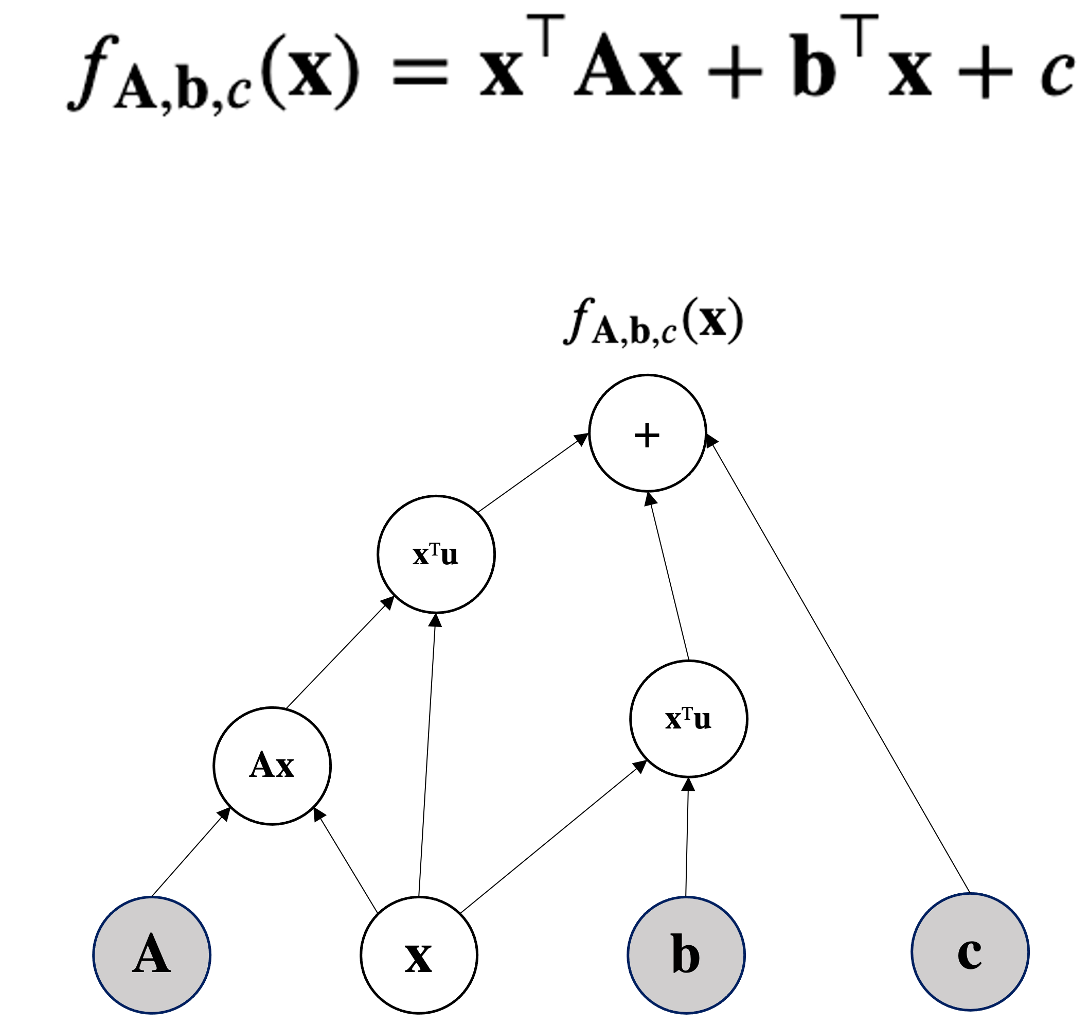
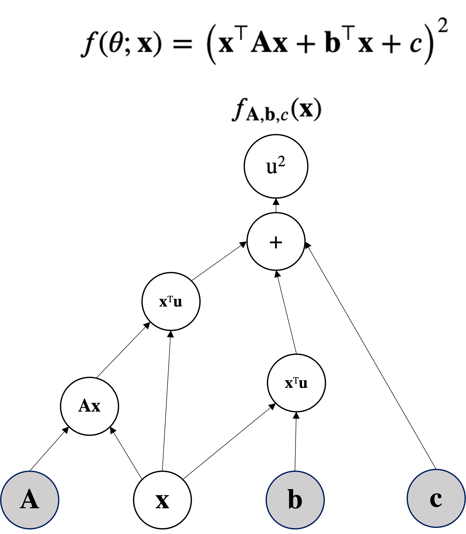
def function(x, thetas):
    A, b, c = thetas
    return torch.pow(x.T @ A @ x + b.T@x + c, 2)
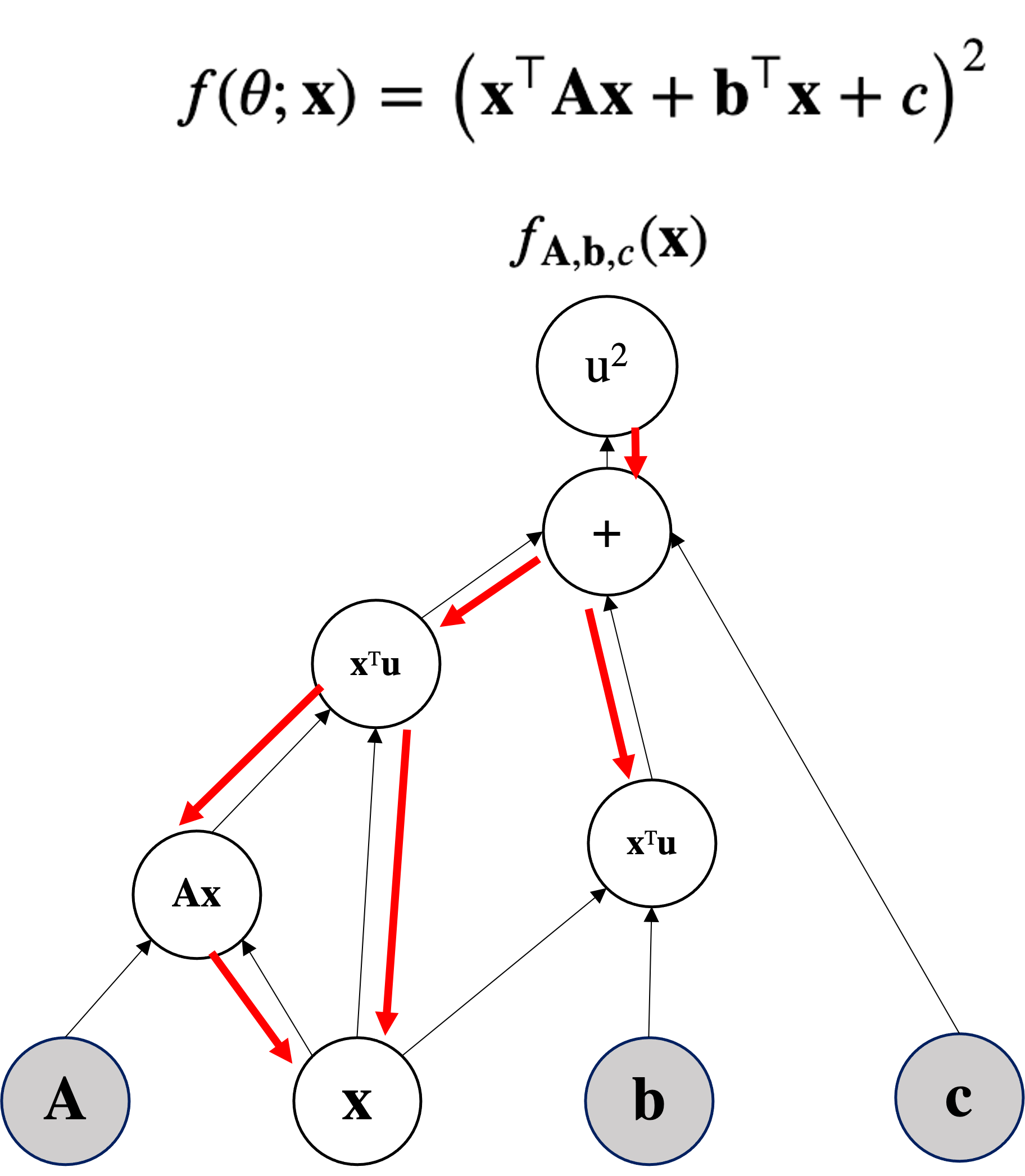
for epoch in range(200):
    if x.grad is not None: x.grad.zero_() # zeroing the gradient before backprop
    func_v = function(x, thetas) # eval function and track gradients (autograd)
    func_v.backward() # get the grads
    if epoch % 20 == 0:
        print(f'{epoch}) y before SGD = ',func_v.item(),'input x=',x.detach().numpy())
    with torch.no_grad(): # here we DO not track gradient
        x += -1e-3*x.grad # plain SGD
        if epoch % 20 == 0:
            print(f'{epoch}) y after SGD  = ',function(x,thetas).item(),
                  'input x=',x.detach().numpy())
0) y before SGD =  4.0 input x= [1. 1.]
0) y after SGD  =  3.5006706714630127 input x= [0.986 0.982]
20) y before SGD =  0.4590446949005127 input x= [0.84928155 0.79601455]
20) y after SGD  =  0.4189494550228119 input x= [0.8456445 0.7907337]
40) y before SGD =  0.08419127017259598 input x= [0.802158  0.7256682]
40) y after SGD  =  0.07775045186281204 input x= [0.80076367 0.72351605]
60) y before SGD =  0.018030276522040367 input x= [0.78288543 0.6954951 ]
60) y after SGD  =  0.01672857254743576 input x= [0.7822726 0.6945199]
80) y before SGD =  0.0041193654760718346 input x= [0.77417433 0.68153346]
80) y after SGD  =  0.0038299155421555042 input x= [0.7738886  0.68107176]
100) y before SGD =  0.000969333981629461 input x= [0.7700594 0.6748613]
100) y after SGD  =  0.0009021023870445788 input x= [0.76992244 0.6746384 ]
120) y before SGD =  0.0002313051954843104 input x= [0.7680748 0.6716252]
120) y after SGD  =  0.00021535974519792944 input x= [0.7680083  0.67151654]
140) y before SGD =  5.5571563279954717e-05 input x= [0.767108  0.6700446]
140) y after SGD  =  5.1754243031609803e-05 input x= [0.76707554 0.6699914 ]
160) y before SGD =  1.3398824194155168e-05 input x= [0.76663494 0.6692699 ]
160) y after SGD  =  1.2477918062359095e-05 input x= [0.766619  0.6692438]
180) y before SGD =  3.2350690162274987e-06 input x= [0.76640296 0.66888946]
180) y after SGD  =  3.0142657578835497e-06 input x= [0.76639515 0.66887665]

function(x, thetas).item()
7.811336786289758e-07
x.T @ A @ x + b.T@x + c
tensor([0.0009], grad_fn=<AddBackward0>)
x
tensor([0.7663, 0.6687], requires_grad=True)
The point $\mbf{x}=[0.7815, 0.7137]$ satisfies approximatively $\mbf{x}^\top\mbf{A}\mbf{x} + \mbf{b}^\top\mbf{x} + c \approx 0 \quad (0.1971)$
with torch.no_grad(): # we do not track the backward pass
    code that uses the function...
In the DAG we only do topological sorting forwarding (no backward).
with torch.no_grad():
    f = function(x, thetas)
print(f, '\n\n-->if you see in the tensor, there is NO grad_fn=<AddBackward0>) as before')
tensor([7.8113e-07])

-->if you see in the tensor, there is NO grad_fn=<AddBackward0>) as before
from torch import nn, optim

model = resnet18(weights=ResNet18_Weights.DEFAULT)

# Freeze all the parameters in the network
for param in model.parameters():
    param.requires_grad = False
def function(x, thetas):
    A, b, c = thetas
    quad = x.T @ A @ x
    linear_detached = (b.T@x).detach() # detaching b*x
    return torch.pow( quad + linear_detached + c, 2)
The high school way
$$\frac{\partial\mathcal{L}(x,y,z)}{\partial x} = ?$$The high school way (as we did until now):
$$\frac{\partial\mathcal{L}(x,y,z)}{\partial x} = (\mbf{x}z+yz)^{\prime}=(\mbf{x}z)^{\prime}+(yz)^{\prime} = z$$$$\frac{\partial\mathcal{L}(x,y,z)}{\partial y} = (xz+\mbf{y}z)^{\prime}=(xz)^{\prime}+(\mbf{y}z)^{\prime} = z$$$$\frac{\partial\mathcal{L}(x,y,z)}{\partial z} = x+y $$but we can re-write it with the chain rule:
$$\frac{\partial\mathcal{L}(x,y,z)}{\partial x} = \big(\underbrace{(\mbf{x}+y)}_{q}z\big)^{\prime}=\frac{\partial\mathcal{L}}{\partial q}\frac{\partial q}{\partial x}$$but we can re-write it with the chain rule:
$$\frac{\partial\mathcal{L}(x,y,z)}{\partial x} = \big(\underbrace{(\mbf{x}+y)}_{q}z\big)^{\prime}=\frac{\partial\mathcal{L}}{\partial q}\frac{\partial q}{\partial x} = z\frac{\partial q}{\partial x} $$but we can re-write it with the chain rule:
$$\frac{\partial\mathcal{L}(x,y,z)}{\partial x} = \big(\underbrace{(\mbf{x}+y)}_{q}z\big)^{\prime}=\frac{\partial\mathcal{L}}{\partial q}\frac{\partial q}{\partial x} = z\cdot 1= z $$The computer science way:

Even if the problem is very small, we break it down to subproblems so that we can automate it:
Who is input of $\mathcal{L}$?
$q$ and $z$ are input of $\mathcal{L}$. $$\frac{\partial\mathcal{L}}{\partial q}, \frac{\partial\mathcal{L}}{\partial z}$$
Even if the problem is very small, we break it down to subproblems so that we can automate it:
What is the derivate? (Just check the operation at the gate) $$\frac{\partial\mathcal{L}}{\partial q}, \frac{\partial\mathcal{L}}{\partial z}$$
Even if the problem is very small, we break it down to subproblems so that we can automate it:
What is the derivate? (Just check the operation at the gate)? $$\frac{\partial\mathcal{L}}{\partial q}=z, \frac{\partial\mathcal{L}}{\partial z}=q$$
Even if the problem is very small, we break it down to subproblems so that we can automate it:
What is the derivative? (Just check the operation at the gate)? $$\frac{\partial\mathcal{q}}{\partial x}=1, \frac{\partial\mathcal{q}}{\partial y}=1$$
Even if the problem is very small, we break it down to subproblems so that we can automate it:
OK now we have all the analytical "local" partial derivatives, we can compute something
$$\frac{\partial\mathcal{L}}{\partial q}=z, \frac{\partial\mathcal{L}}{\partial z}=q, \frac{\partial\mathcal{q}}{\partial x}=1, \frac{\partial\mathcal{q}}{\partial y}=1$$
OK now we have all the analytical partial derivatives, we can compute something
$$\frac{\partial\mathcal{L}}{\partial q}=z, \frac{\partial\mathcal{L}}{\partial z}=q, \frac{\partial\mathcal{q}}{\partial x}=1, \frac{\partial\mathcal{q}}{\partial y}=1$$
OK now we have all the analytical partial derivatives, we can compute something
$$\frac{\partial\mathcal{L}}{\partial q}=z, \frac{\partial\mathcal{L}}{\partial z}=q, \frac{\partial\mathcal{q}}{\partial x}=1, \frac{\partial\mathcal{q}}{\partial y}=1$$
This is what we wanted: $$\frac{\partial\mathcal{L}}{\partial x},\frac{\partial\mathcal{L}}{\partial y},\frac{\partial\mathcal{L}}{\partial z}$$
This is what we have
$$\frac{\partial\mathcal{L}}{\partial q}=z, \frac{\partial\mathcal{L}}{\partial z}=q, \frac{\partial\mathcal{q}}{\partial x}=1, \frac{\partial\mathcal{q}}{\partial y}=1$$
Act as a base case for the recursion: $$\frac{\partial\mathcal{L}}{\partial \mathcal{L}}=?$$
This is what we wanted: $$\frac{\partial\mathcal{L}}{\partial x},\frac{\partial\mathcal{L}}{\partial y},\frac{\partial\mathcal{L}}{\partial z}$$
This is what we have
$$\frac{\partial\mathcal{L}}{\partial q}=z, \frac{\partial\mathcal{L}}{\partial z}=q, \frac{\partial\mathcal{q}}{\partial x}=1, \frac{\partial\mathcal{q}}{\partial y}=1$$
Act as a base case for the recursion: $$\frac{\partial\mathcal{L}}{\partial \mathcal{L}}=1$$
This is what we wanted: $$\frac{\partial\mathcal{L}}{\partial x},\frac{\partial\mathcal{L}}{\partial y},\frac{\partial\mathcal{L}}{\partial z}$$
This is what we have
$$\frac{\partial\mathcal{L}}{\partial q}=z, \frac{\partial\mathcal{L}}{\partial z}=q, \frac{\partial\mathcal{q}}{\partial x}=1, \frac{\partial\mathcal{q}}{\partial y}=1$$
What is the value of the gradient of $\mathcal{L}$ on $z$?:
$$\frac{\partial\mathcal{L}}{\partial z}= q = 3$$This is what we wanted: $$\frac{\partial\mathcal{L}}{\partial x},\frac{\partial\mathcal{L}}{\partial y},\frac{\partial\mathcal{L}}{\partial z}$$
This is what we have
$$\frac{\partial\mathcal{L}}{\partial q}=z, \frac{\partial\mathcal{L}}{\partial z}=q, \frac{\partial\mathcal{q}}{\partial x}=1, \frac{\partial\mathcal{q}}{\partial y}=1$$
What is the value of the gradient of $\mathcal{L}$ on $q$?:
This is what we wanted: $$\frac{\partial\mathcal{L}}{\partial x},\frac{\partial\mathcal{L}}{\partial y},\frac{\partial\mathcal{L}}{\partial z}$$
This is what we have
$$\frac{\partial\mathcal{L}}{\partial q}=z, \frac{\partial\mathcal{L}}{\partial z}=q, \frac{\partial\mathcal{q}}{\partial x}=1, \frac{\partial\mathcal{q}}{\partial y}=1$$
What is the value of the gradient of $\mathcal{L}$ on $q$?:
$$\frac{\partial\mathcal{L}}{\partial q}= z = -4$$This is what we wanted: $$\frac{\partial\mathcal{L}}{\partial x},\frac{\partial\mathcal{L}}{\partial y},\frac{\partial\mathcal{L}}{\partial z}$$
This is what we have
$$\frac{\partial\mathcal{L}}{\partial q}=z, \frac{\partial\mathcal{L}}{\partial z}=q, \frac{\partial\mathcal{q}}{\partial x}=1, \frac{\partial\mathcal{q}}{\partial y}=1$$
What is the value of the gradient of $\mathcal{L}$ on $y$?:
This is what we wanted: $$\frac{\partial\mathcal{L}}{\partial x},\frac{\partial\mathcal{L}}{\partial y},\frac{\partial\mathcal{L}}{\partial z}$$
This is what we have
$$\frac{\partial\mathcal{L}}{\partial q}=z, \frac{\partial\mathcal{L}}{\partial z}=q, \frac{\partial\mathcal{q}}{\partial x}=1, \frac{\partial\mathcal{q}}{\partial y}=1$$
What is the value of the gradient of $\mathcal{L}$ on $y$?: $$\frac{\partial\mathcal{L}}{\partial y} = \frac{\partial\mathcal{L}}{\partial q}\frac{\partial q}{\partial y} = z\cdot 1= -4$$
This is what we wanted: $$\frac{\partial\mathcal{L}}{\partial x},\frac{\partial\mathcal{L}}{\partial y},\frac{\partial\mathcal{L}}{\partial z}$$
This is what we have
$$\frac{\partial\mathcal{L}}{\partial q}=z, \frac{\partial\mathcal{L}}{\partial z}=q, \frac{\partial\mathcal{q}}{\partial x}=1, \frac{\partial\mathcal{q}}{\partial y}=1$$
The high school way (as we did until now):
$$\frac{\partial\mathcal{L}(x,y,z)}{\partial x} = (\mbf{x}z+yz)^{\prime}=(\mbf{x}z)^{\prime}+(yz)^{\prime} = z = -4$$$$\frac{\partial\mathcal{L}(x,y,z)}{\partial y} = (xz+\mbf{y}z)^{\prime}=(xz)^{\prime}+(\mbf{y}z)^{\prime} = z = -4$$$$\frac{\partial\mathcal{L}(x,y,z)}{\partial z} = x+y = +3 $$from torch import tensor
def neural_net(x,y,z):
return (x+y)*z
x, y, z = tensor(-2., requires_grad=True), tensor(5.,requires_grad=True), tensor(-4., requires_grad=True)
loss = neural_net(x,y,z) # forward pass
loss.backward() # backward (after this I can check the gradients)
for el in [x,y,z]:
print(el.grad)
tensor(-4.)
tensor(-4.)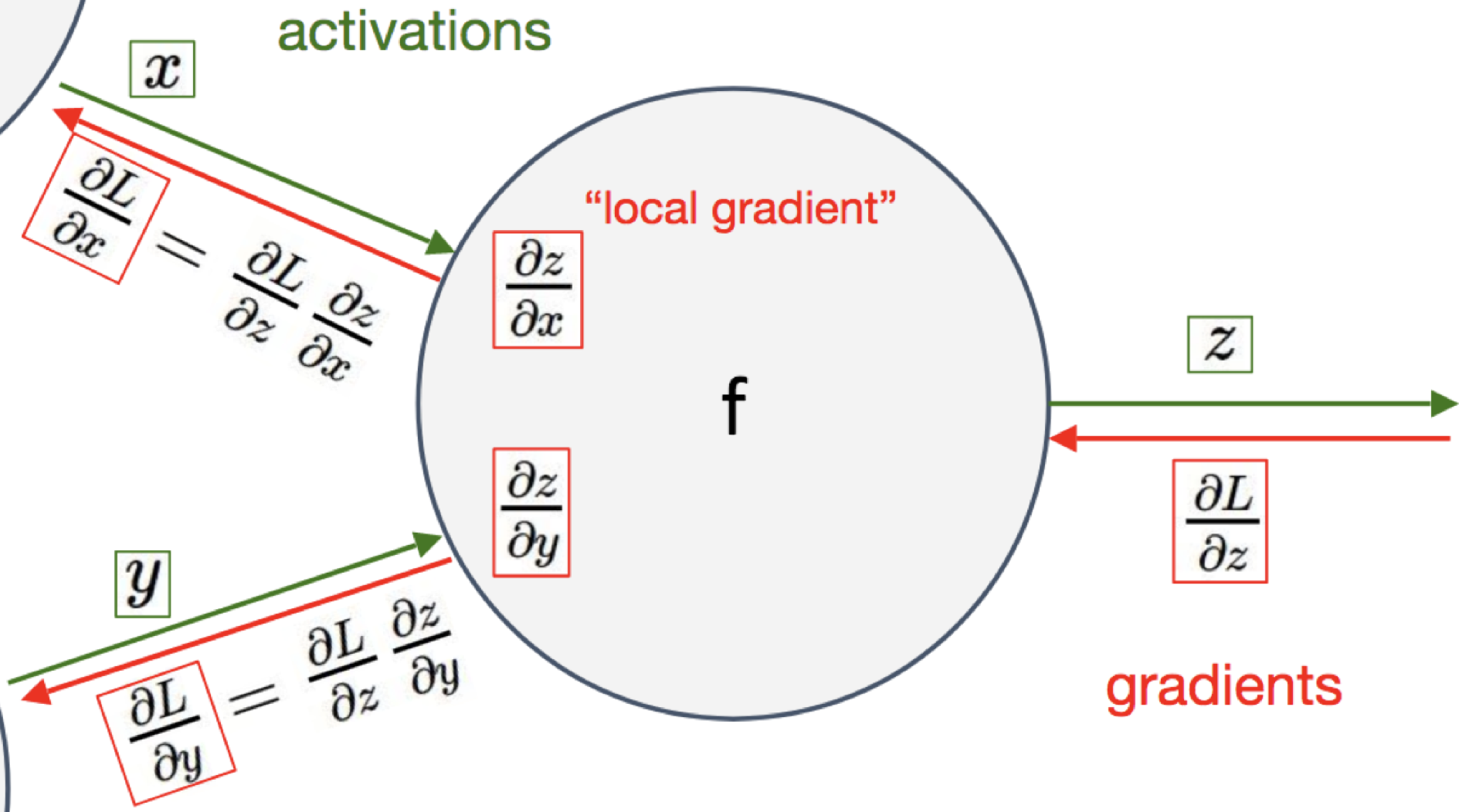
tensor(3.)Just remember that you have to do at a generic gate:
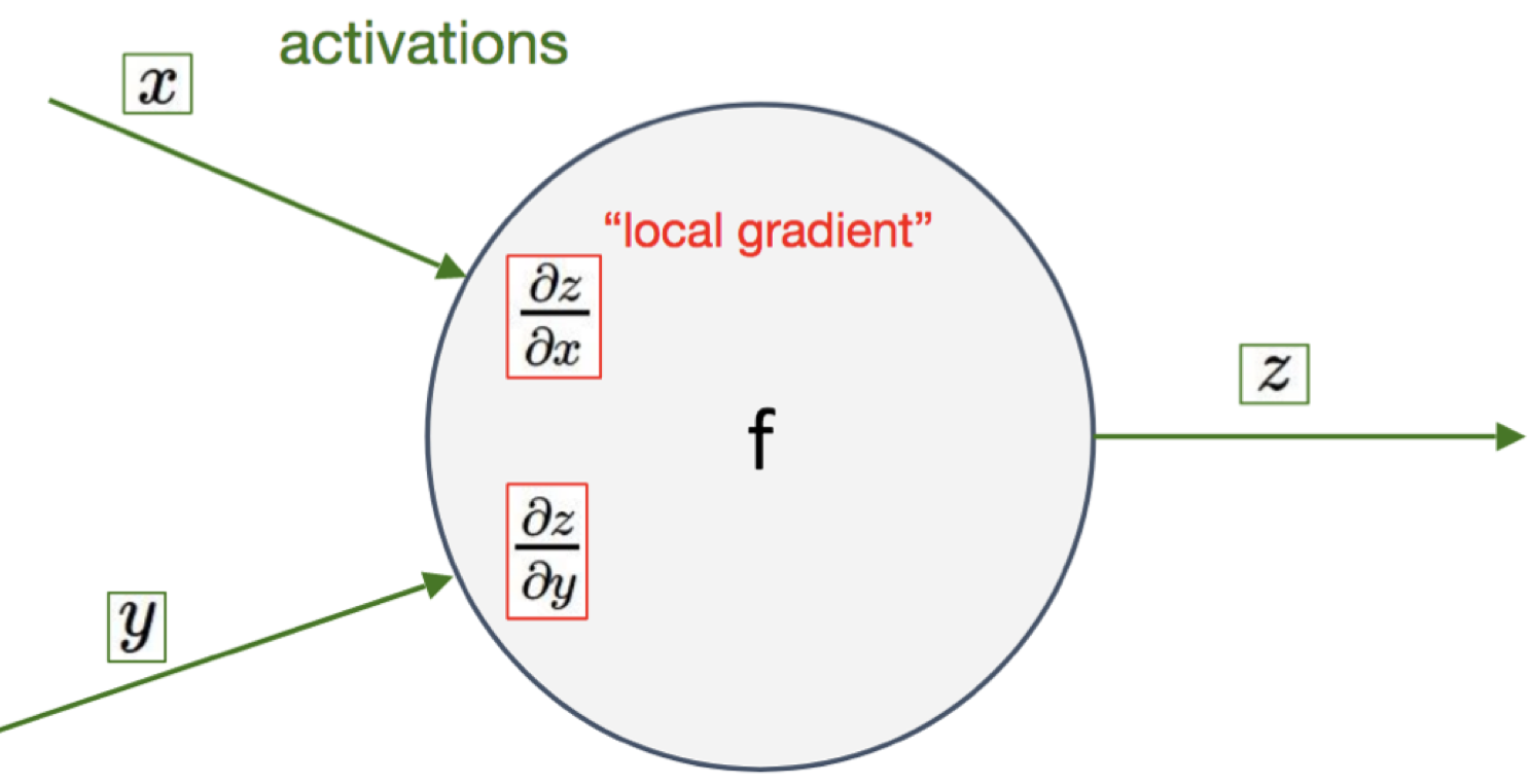
Multiply the gradient that you receive with your local gradient
Given the above function, can you perform forward and backward pass by writing all the local values and local gradient, by applying the chain rule?
(Direct computation of the gradient does not count for solving it, though you may be using it to double check)

This is what implements the Sigmoid Layer in Pytorch:

$\forall l \in [1\ldots,L]$:

Below we take the partial derivative wrt class j, so it is not in vector notation:
$$\partial_{z_j} \mathcal{L}(\mathbf{y}, \hat{\mathbf{y}}) = \frac{\exp(z_j)}{\sum_{k=1}^q \exp(z_k)} - y_j = \mathrm{softmax}(\mathbf{z})_j - y_j$$It is a GLM!
Below we take the partial derivative wrt class j, so it is not in vector notation:
$$\partial_{z_j} \mathcal{L}(\mathbf{y}, \hat{\mathbf{y}}) = \frac{\exp(z_j)}{\sum_{k=1}^q \exp(z_k)} - y_j = \mathrm{softmax}(\mathbf{z})_j - y_j$$p = [0.2 0.7 0.1] y =[0 1 0]
dL/dz = [0.2 0.7-1 0.1] = [0.2 -0.3 0.1]
$\forall l \in [1\ldots,L]$:

Part of these lectures are taken from:
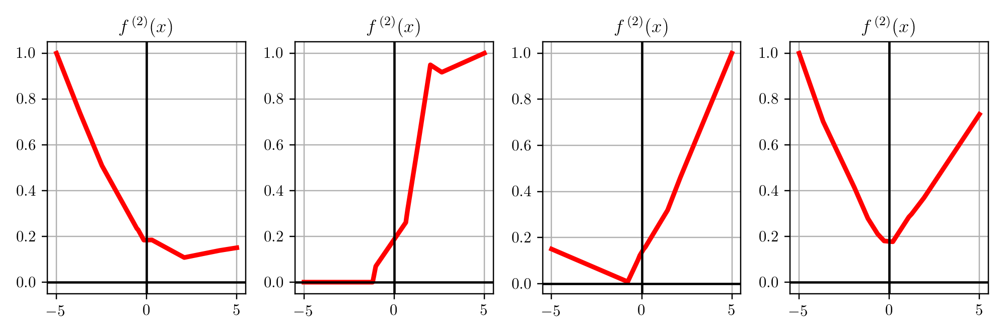
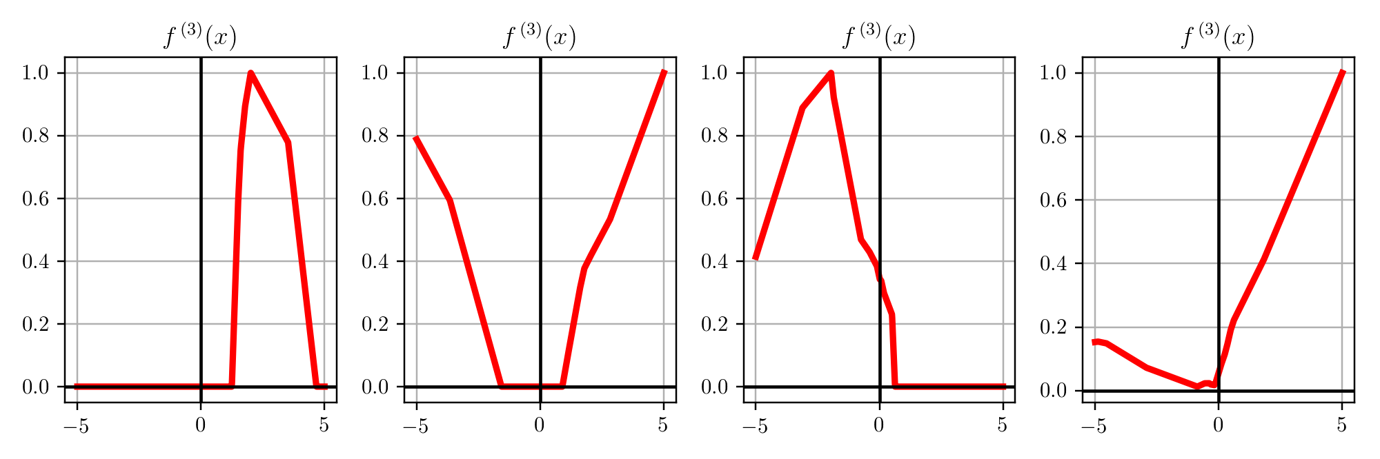
Second Derivative: $f(x)^{\prime\prime}$: $\mathbb{R}^{d\times d \times p}$ Tensor of second derivative (high order tensor)
Informally: a tensor is a generalization of matrices in N-D dimensions
256x256 images you get Nx256x256 which is a tensor.x_big = np.arange(0.01, 3.01, 0.01)
ys = np.sin(x_big**x_big)
_ = plt.plot(x_big, ys, 'b-')
plt.xlabel('x');plt.ylabel('y');
_ = plt.axis('equal')

x_med = np.arange(1.75, 2.25, 0.001)
ys = np.sin(x_med**x_med)
_ = plt.plot(x_med, ys, 'b-')
plt.xlabel('x');plt.ylabel('y');
_ = plt.axis('equal')

Taking this to an extreme, if we zoom into a tiny segment, the behavior becomes far simpler: it is just a straight line.
x_small = np.arange(2.0, 2.01, 0.0001)
ys = np.sin(x_small**x_small)
_ = plt.plot(x_small, ys, 'b-')
plt.xlabel('x');plt.ylabel('y');
_ = plt.axis('equal')

Thus, we can consider the ratio of the change in the output of a function for a small change in the input of the function. We can write this formally as
$$ \frac{L(x+\epsilon) - L(x)}{(x+\epsilon) - x} = \frac{L(x+\epsilon) - L(x)}{\epsilon}. $$Different texts will use different notations for the derivative. For instance, all of the below notations indicate the same thing:
$$ \frac{df}{dx} = \frac{d}{dx}f = f' = \nabla_xf = D_xf = f_x. $$When working with derivatives, it is often useful to geometrically interpret the approximation used above. In particular, note that the equation
$$ f(x+\epsilon) \approx f(x) + \epsilon \frac{df}{dx}(x), $$Approximates the value of $f$ by:
in a neighbourhood $[-\epsilon,+\epsilon]$
In this way we say that the derivative gives a linear approximation to the function $f$, as illustrated below:

$\def\der#1#2{\frac{\partial #1}{\partial #2}}$ $\def\derr#1#2#3{\frac{\partial^2 #1}{\partial#2\partial #3}}$
Geometric Interpretation
The direction to change the input so that the function values go up in $[x,x+\epsilon]$
$$f\Big(\mbf{x} + \epsilon\nabla_{\mbf{x}}f(\mbf{x})\Big) \ge f(\mbf{x})$$

The gradient, represented by the blue arrows, denotes the direction of greatest change of a scalar function. The values of the function are represented in grayscale and increase in value from white (low) to dark (high).
Figure credit Wikipedia
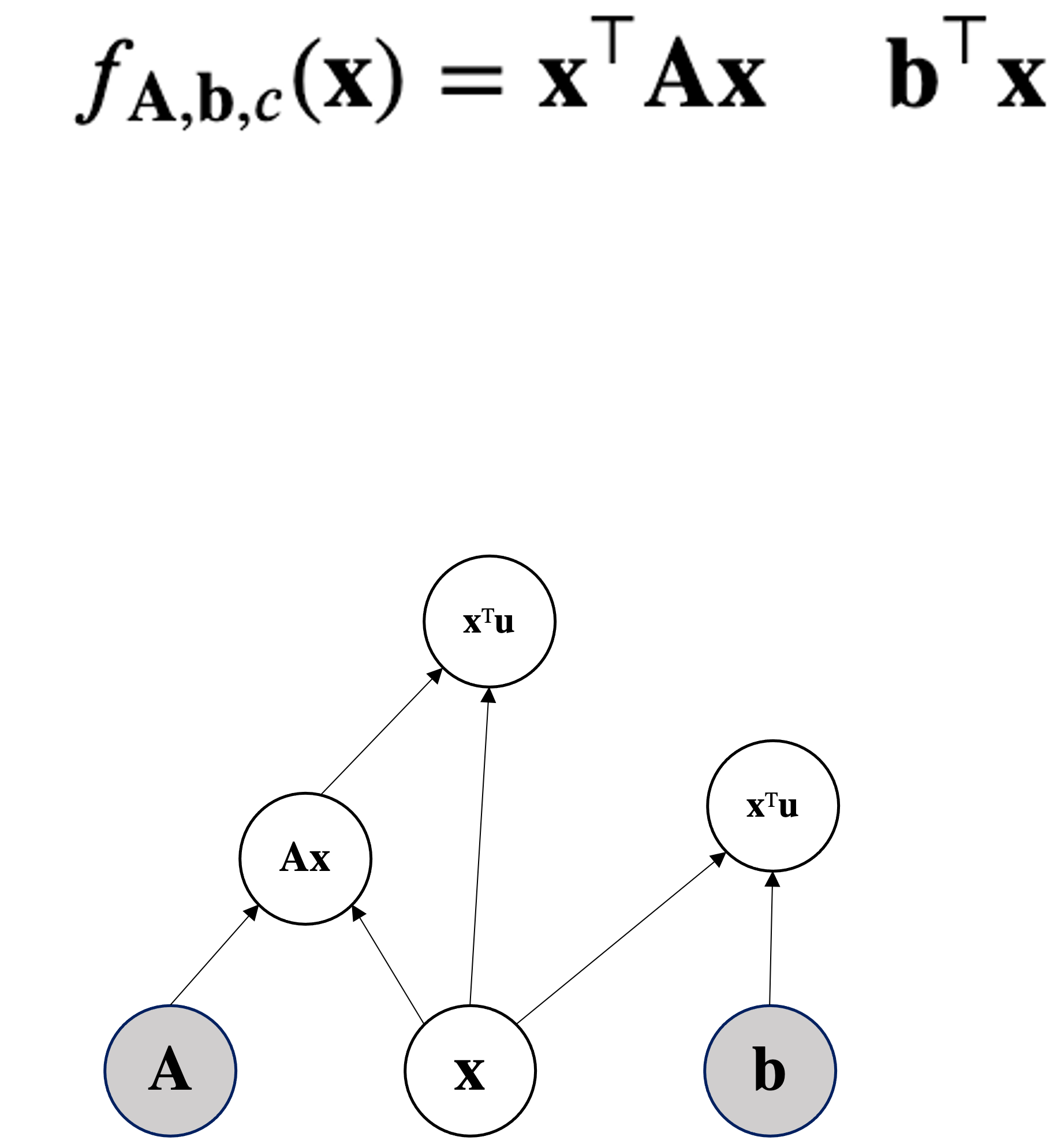
Given the function $f(\mbf{x};\mbf{b})= \mbf{b}^T\mbf{x}$ parametrized by the vector $\mbf{b}$ that takes as input a vector $\mbf{x}$—both vectors in $\mathbb{R}^d$—compute the gradient of x $$\nabla_\mbf{x} f(\mbf{x}) = \nabla_\mbf{x} \mbf{b}^T\mbf{x}$$
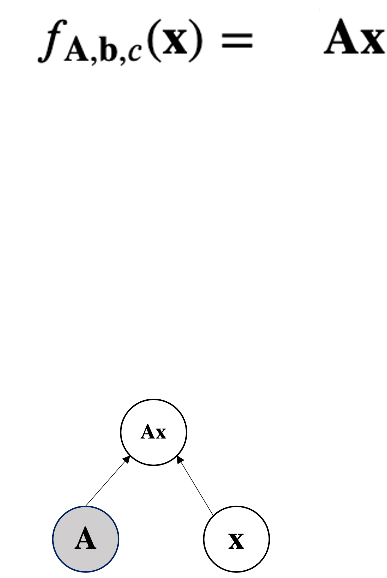
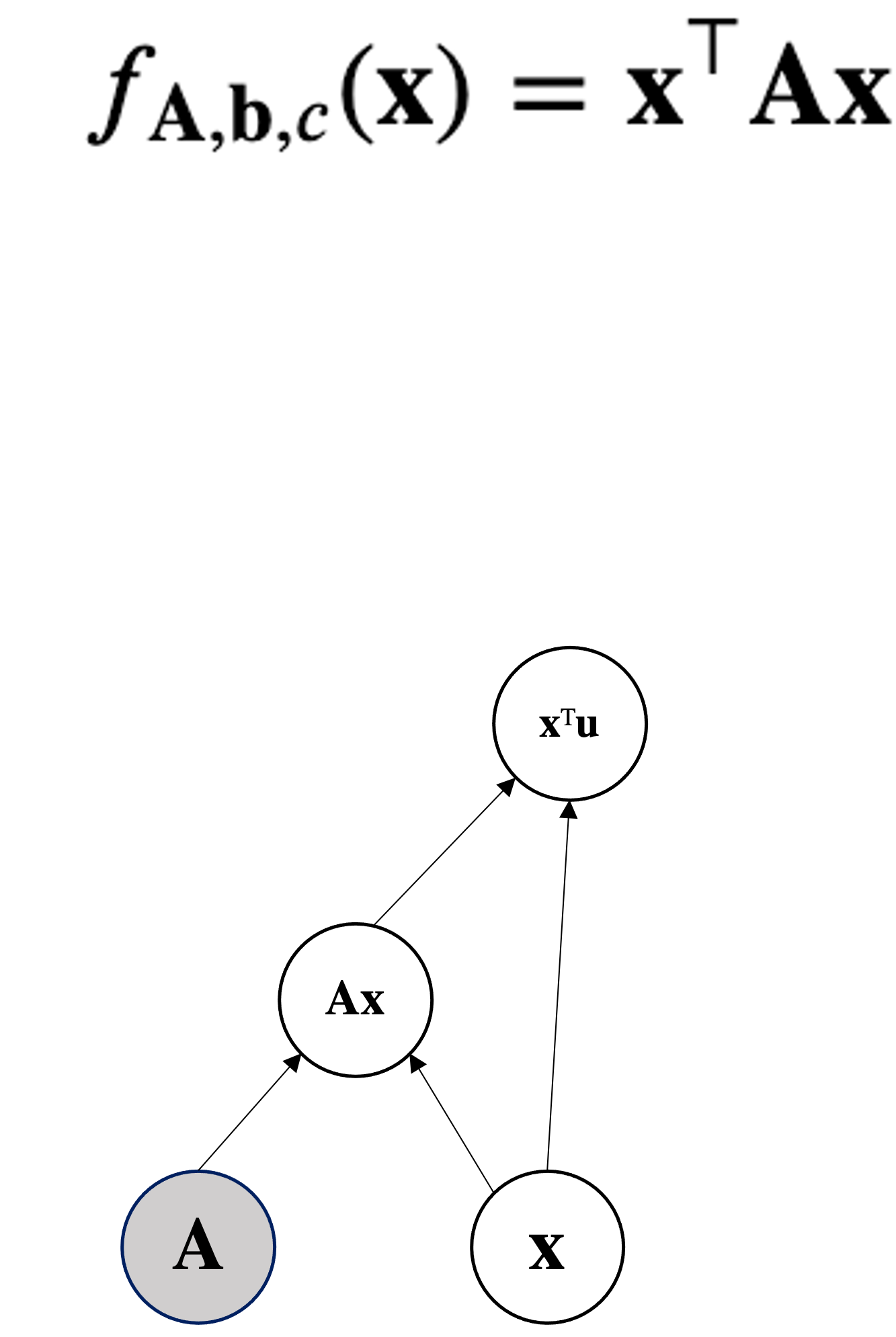
Given $\mbf{A} \in \mathbb{R}^{d\times d}$ symmetric and square and $\mbf{x} \in \mathbb{R}^d$ then a quadratic form is: $$\mbf{x}^T \mbf{A}\mbf{x}$$
$\forall \mbf{x} \neq 0 \qquad \mbf{x}^T \mbf{A}\mbf{x} \le 0 $ is negative semi-definite (NSD) - Relation with eigenvalues all non-positive
$\forall \mbf{x} \neq 0 \qquad \mbf{x}^T \mbf{A}\mbf{x} \lt, \gt 0 $ is indefinite - Relation with eigenvalues mixed in sign

Compute $\nabla_{\mbf{x}}\mbf{x}^T\mbf{A}\mbf{x}$.
Can be seen as $\mbf{x}^T\mbf{f(x)}$ where $\mbf{f(x)} = \mbf{A}\mbf{x}$