Machine Learning

Machine Learning

---

7. Linear Regression

Prof. Iacopo Masi - Computer Science Department, Sapienza University of Rome

Recap previous lecture

• Model Selection and Assessment
• Cross-validation
• Evaluation Metrics

Today's lecture

We go back to your loved 🥰 Linear Algebra

Supervised, Parametric Models

1) Ordinary Linear Regression with Least Squares

2) Probabilistic Interpretation

3) Gradient Descent "Family"

This lecture material is taken from

• Mostly from Stanford class
• Stanford notes
• Tibshirani - Chapter 4 page 43
• Sklearn model selection
• Bishop - Chapter 3 page 137

import numpy as np
from matplotlib import pyplot as plt

from sklearn import linear_model, datasets


n_samples = 100
size = 10

X, y, coef_gt = datasets.make_regression(
    n_samples=n_samples,
    n_features=2,
    n_informative=1,
    noise=20,
    coef=True,
    random_state=42,
)
fig = plt.figure(figsize=(size, size))
ax = fig.add_subplot(projection='3d')
ax.scatter(X[..., 0], X[..., 1], y, c='red', marker='o')
ax.view_init(0, -90)

import numpy as np
from matplotlib import pyplot as plt

from sklearn import linear_model, datasets


n_samples = 100
size = 10

X, y, coef_gt = datasets.make_regression(
    n_samples=n_samples,
    n_features=2,
    n_informative=1,
    noise=20,
    coef=True,
    random_state=42,
)
fig = plt.figure(figsize=(size, size))
ax = fig.add_subplot(projection='3d')
ax.scatter(X[..., 0], X[..., 1], y, c='red', marker='o')
ax.view_init(0, -90)

The data

x_1	x_2	y
-1.415	-0.420	-116.6
0.5219	0.2969	58.737
-0.889	-0.815	-73.89
-0.883	0.1537	-113.3
0.7384	0.1713	63.998
-0.264	2.7201	-30.33
1.1428	0.7519	81.616
0.3613	1.5380	48.283
0.8125	1.3562	119.06
-0.223	0.7140	-12.36
-1.106	-1.196	-122.4

Living area vs Apartment Price

Linear Regression settings

We want to regress $y$ from $\mbf{x}$ that is we want to learn a function $f_{\boldsymbol{\theta}}$ parametrized by some parameters $\boldsymbol{\theta}$ so that $ f_{\boldsymbol{\theta}}: \underbrace{\mbf{x}}_{\text{input}} \mapsto \underbrace{y}_{\text{output}}$

• $\mbf{x} \in \mathbb{R}^d$ (here d=2)
• $y$ is a scalar that is continuous $y \in \mathbb{R}$
• We have a finite number of samples $D = \{\mbf{x}_i,y_i\}_{i=1}^n \sim p(\mbf{x},y)$ that which labels are generated from a function $f$ plus error so $y = f(\mbf{x}) + \epsilon$

Linear Hypothesis

We assume the relation $f \longleftrightarrow y$ is linear.

We know $D = \{\mbf{x}_i,y_i\}_{i=1}^n$ and we want to find ${\boldsymbol{\theta}}\doteq (\theta_0,\ldots,\theta_d)$

$$ f_{\boldsymbol{\theta}}(\mbf{x}) = \theta_0+ \theta_1\cdot x_1 + \theta_2\cdot x_2 + \ldots + \theta_d\cdot x_d$$

So ${\boldsymbol{\theta}}\doteq (\theta_0,\ldots,\theta_d) \in \mathbb{R}^{d+1}$.

$$ f_{\boldsymbol{\theta}}(\mbf{x}) = \big(\sum_{i=1}^d\theta_i\cdot x_i\big) + \theta_0$$

Trick for Notation Compactness

We can augment each feature to have a bias (intercept term) set to $1$ so that $\mbf{x} \doteq [1,\mbf{x}]$.

Doing so $\mbf{x} \in \mathbb{R}^{d+1}$

$$ f_{\boldsymbol{\theta}}(\mbf{x}) = \theta_0\cdot \underbrace{x_0}_{\text{always}~1} + \theta_1\cdot x_1 + \theta_2\cdot x_2 + \ldots + \theta_d\cdot x_d$$

So ${\boldsymbol{\theta}}\doteq (\theta_0,\ldots,\theta_d) \in \mathbb{R}^{d+1}$.

$$ f_{\boldsymbol{\theta}}(\mbf{x}) = \sum_{i=0}^d\theta_i\cdot x_i = \bmf{\theta}^T\mbf{x} $$

Parametric Nature

No matter how many training points $N$ you have, the parameters are fixed in $\bmf{\theta}$.

Note that $\bmf{\theta} \in \mathbb{R}^{d+1}$.

$$ f_{\boldsymbol{\theta}}(\mbf{x}) = \sum_{i=0}^d\theta_i\cdot x_i = \bmf{\theta}^T\mbf{x} $$

Loss or Cost Function for Linear Regression

You see now that the loss is more explicit compared to non-parametric models (K-NN, Decision Trees).

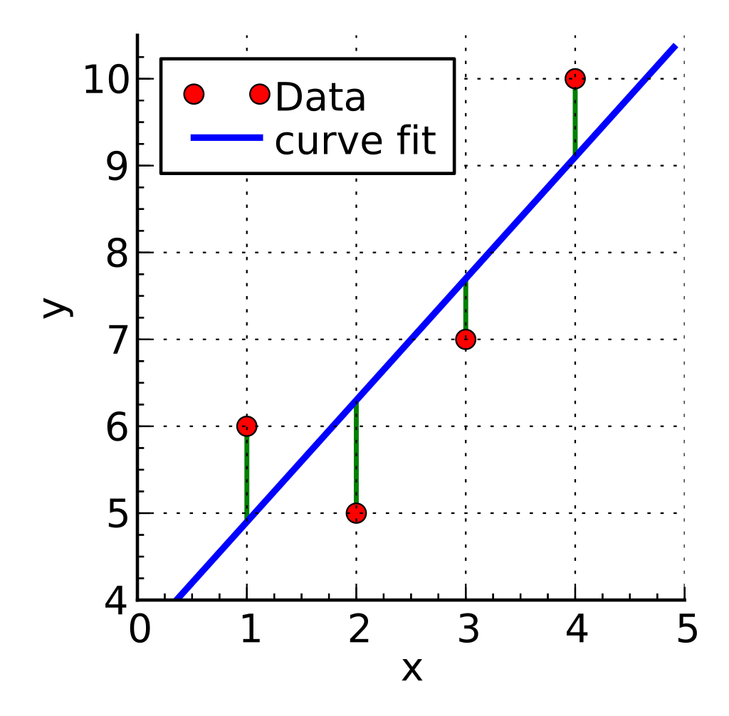
$$ \mathcal{J}(\mbf{\theta};\mbf{x},y)= \frac{1}{2} \sum_{i=1}^{n}\mathcal{L}\big(y_{i}, f_{\boldsymbol{\theta}}(\mbf{x}_i)\big)$$

where

$$\mathcal{L}\big(y, f_{\boldsymbol{\theta}}(\mbf{x})\big) = \big(f_{\boldsymbol{\theta}}(\mbf{x}) - y \big)^2 $$

The loss is the squared error.

Minimize the Total Loss with a Closed Form Solution

We need to minimize $$ \mathcal{J}(\mbf{\theta};\mbf{x},y)= \frac{1}{2} \sum_{i=1}^{n}\mathcal{L}\big(y_{i}, f_{\boldsymbol{\theta}}(\mbf{x}_i)\big)$$ so to find:

$$\mbf{\theta}^{\star} = \arg\min_{\mbf{\theta}} \mathcal{J}(\mbf{\theta};\mbf{x},y) $$

Explicit Cost

$$ \mathcal{J}(\mbf{\theta};\mbf{x},y)= \frac{1}{2} \sum_{i=1}^{n} (\underbrace{\bmf{\theta}^T\mbf{x}_i}_{f_{\boldsymbol{\theta}}} - y_i)^2$$

Vectorizing the Explicit Cost

$$ \mathcal{J}(\mbf{\theta};\mbf{x},y)= \frac{1}{2} \sum_{i=1}^{n} (\underbrace{\bmf{\theta}^T\mbf{x}_i}_{f_{\boldsymbol{\theta}}} - y_i)^2$$

We define the design matrix $\mbf{X} \in \mathbb{R}^{n\times (d+1)}$ and label matrix $\mbf{y}\in \mathbb{R}^{n\times 1} $

$$ \def\horzbar{\rule[.5ex]{2.5ex}{0.5pt}} \mbf{X} = \left[ \begin{array}{ccc} \horzbar & \mbf{x}^{T}_{1} & \horzbar \\ \horzbar & \mbf{x}^{T}_{2} & \horzbar \\ & \vdots & \\ \horzbar & \mbf{x}^{T}_{n} & \horzbar \end{array} \right] \; \qquad \mbf{y} = \left[ \begin{array}{c} {y}_{1} \\ {y}_{2} \\ \vdots \\ {y}_{n} \\ \end{array} \right] $$

The parameters $\bmf{\theta} \in \mathbb{R}^{d+1}$ are:

$$ \bmf{\theta} = \left[ \begin{array}{c} \theta_{0} \\ \theta_{1} \\ \vdots \\ \theta_{d} \\ \end{array} \right] $$

Vectorizing the Explicit Cost

$$ \underbrace{\mbf{X}}_{\mathbb{R}^{n\times (d+1)}} \underbrace{\bmf{\theta}}_{\mathbb{R}^{(d+1)\times1}} - \underbrace{\mbf{y}}_{\mathbb{R}^{n}}$$

$$ \underbrace{\mbf{X} \bmf{\theta}}_{\mathbb{R}^{n}} - \underbrace{\mbf{y}}_{\mathbb{R}^{n}}$$$$ \mbf{X}\bmf{\theta} - \mbf{y} = \left[ \begin{array}{ccc} & \mbf{x}^{T}_{1}\bmf{\theta} - y_1 & \\ & \mbf{x}^{T}_{2}\bmf{\theta} - y_2 & \\ & \vdots & \\ & \mbf{x}^{T}_{n}\bmf{\theta} - y_n & \end{array} \right] $$

Vectorizing the Explicit Cost

$$\mathcal{J}(\mbf{\theta};\mbf{X},\mbf{y})= \frac{1}{2} \big(\mbf{X}\bmf{\theta} - \mbf{y} \big)^T\big(\mbf{X}\bmf{\theta} - \mbf{y} \big) = \frac{1}{2} \sum_{i=1}^{n} (\underbrace{\bmf{\theta}^T\mbf{x}_i}_{f_{\boldsymbol{\theta}}} - y_i)^2$$

Solve it

Set the gradient to zero to find critical points:

$$\nabla_{\mbf{\theta}} \mathcal{J}(\mbf{\theta};\mbf{X},\mbf{y}) = 0$$

$$\nabla_{\mbf{\theta}} \frac{1}{2} \big(\mbf{X}\bmf{\theta} - \mbf{y} \big)^T\big(\mbf{X}\bmf{\theta} - \mbf{y} \big) = 0 $$

For now forget the "equal to zero":

$$\nabla_{\mbf{\theta}} \frac{1}{2} \big[ (\mbf{X}\bmf{\theta})^T(\mbf{X}\bmf{\theta}) - \underbrace{(\mbf{X}\bmf{\theta})^T\mbf{y}}_{\text{scalar}} - \underbrace{\mbf{y}^T(\mbf{X}\bmf{\theta})}_{\text{scalar}} + \mbf{y}^T\mbf{y}) \big] $$

$$\nabla_{\mbf{\theta}} \frac{1}{2} \big[ (\mbf{X}\bmf{\theta})^T(\mbf{X}\bmf{\theta}) - 2\bmf{\theta}^T(\mbf{X}^T\mbf{y}) + \mbf{y}^T\mbf{y}) \big] $$

$$\nabla_{\mbf{\theta}} \frac{1}{2} \big[ \bmf{\theta}^T(\mbf{X}^T\mbf{X})\bmf{\theta} - 2\bmf{\theta}^T(\mbf{X}^T\mbf{y}) + \mbf{y}^T\mbf{y}) \big] $$

$$ \frac{1}{2} \big[ 2\mbf{X}^T\mbf{X}\bmf{\theta} - 2\mbf{X}^T\mbf{y} \big]$$

Set the gradient to zero

$$ \frac{1}{2} \big[ 2\mbf{X}^T\mbf{X}\bmf{\theta} - 2\mbf{X}^T\mbf{y} \big] = 0$$

To get the normal equation

$$\mbf{X}^T\mbf{X}\bmf{\theta} = \mbf{X}^T\mbf{y}$$

Final Least Squares solution

Assumes $\mbf{X}^T\mbf{X}$ is invertible:

$$\bmf{\theta} = \underbrace{(\mbf{X}^T\mbf{X})^{-1}\mbf{X}^T}_{\text{pseudo inverse}}\mbf{y} = \mbf{X}^{+}\mbf{y}$$

where:

$$ \mbf{X}^{+} \doteq (\mbf{X}^T\mbf{X})^{-1}\mbf{X}^T$$

%matplotlib notebook
from sklearn import linear_model, datasets
from matplotlib import pyplot as plt
import numpy as np

n_samples = 100
size = 8

X, y, coef_gt = datasets.make_regression(
    n_samples=n_samples,
    n_features=2,
    n_informative=1,
    noise=20,
    coef=True,
    random_state=42,
)
fig = plt.figure(figsize=(size, size))
ax = fig.add_subplot(projection='3d')
# Linear Regression
bias = np.ones((X.shape[0], 1))
X = np.hstack((X, bias))
theta = np.linalg.inv(X.T@X)@X.T@y
# Now MeshGrid
Xmin, Xmax = X.min(), X.max()
support = np.linspace(Xmin, Xmax, 10)
xx, yy = np.meshgrid(support, support)
data = np.stack((xx, yy), axis=2)
data = data.reshape(-1, 2)
data = np.hstack((data, np.ones((data.shape[0], 1))))
z = np.dot(theta, data.T)
z = z.reshape(xx.shape)
ax.plot_surface(xx, yy, z, alpha=0.2)
ax.scatter(X[..., 0], X[..., 1], y, c='red', marker='o')
ax.view_init(0, 90)

Debugging the Coefficients

$$ f_{\boldsymbol{\theta}}(\mbf{x}) = \sum_{i=0}^d\theta_i\cdot x_i = \bmf{\theta}^T\mbf{x} $$

%matplotlib inline
plt.figure()
plt.bar(list(range(theta.size)),theta); plt.xlabel('Coefficients');

%matplotlib inline
plt.figure()
plt.bar(list(range(coef_gt.size)),coef_gt); plt.xlabel('Coefficients GT');

Important: The distance is NOT orthogonal

Important: The distance is NOT orthogonal (1D case)

Interpretation as solving an overdetermined Linear System ($n\gg d$)

Assumes $\mbf{X}^T\mbf{X}$ is invertible (full rank) and $n\gg d$:

$$\bmf{\theta} = \underbrace{(\mbf{X}^T\mbf{X})^{-1}}_{d\times d}\underbrace{\mbf{X}^T}_{d\times n}\underbrace{\mbf{y}}_{n\times 1}$$

The normal equation gives you a way to invert $\mbf{X}^T\mbf{X}$

$$\mbf{X}^T\mbf{X}\bmf{\theta} = \mbf{X}^T\mbf{y}$$

it solves the linear system so that the plane best fits all the points with a trade-off given by the square of the residuals (least squares).

What happens if $n=d+1$?

$$\underbrace{\mbf{X}}_{n\times n} \bmf{\theta}= \mbf{y}$$

We can invert it "directly"

$$\bmf{\theta} = \mbf{X}^{-1}\mbf{y}$$

Why? $$ (\mbf{A}\mbf{B})^{-1} = (\mbf{B}^{-1}\mbf{A}^{-1}) $$ then:

$$\bmf{\theta} = (\mbf{X}^T\mbf{X})^{-1}\mbf{X}^T\mbf{y} = \mbf{X}^{-1}(\mbf{X}^T)^{-1}\mbf{X}^T\mbf{y} = \mbf{X}^{-1}\mbf{y}$$

%matplotlib notebook
from sklearn import linear_model, datasets
from matplotlib import pyplot as plt
import numpy as np

n_samples = 3
size = 12

X, y, coef_gt = datasets.make_regression(
    n_samples=n_samples,
    n_features=2,
    n_informative=1,
    noise=20,
    coef=True,
    random_state=42,
)
fig = plt.figure(figsize=(size, size))
ax = fig.add_subplot(projection='3d')
ax.scatter(X[..., 0], X[..., 1], y, c='blue', marker='o')
# Linear Regression
bias = np.ones((X.shape[0], 1))
X = np.hstack((X, bias))
theta = np.linalg.inv(X)@y
# Now MeshGrid
Xmin, Xmax = X.min(), X.max()
support = np.linspace(Xmin, Xmax, 10)
xx, yy = np.meshgrid(support, support)
data = np.stack((xx, yy), axis=2)
data = data.reshape(-1, 2)
data = np.hstack((data, np.ones((data.shape[0], 1))))
z = np.dot(theta, data.T)
z = z.reshape(xx.shape)
ax.plot_surface(xx, yy, z, alpha=0.2)
ax.scatter(X[..., 0], X[..., 1], y, c='red', marker='o')
ax.view_init(0, 90)

What happens if $n=d$?

We see the plane passes exactly through the "training points".

Probabilistic Interpretation

Probabilistic Interpretation for Linear Regression

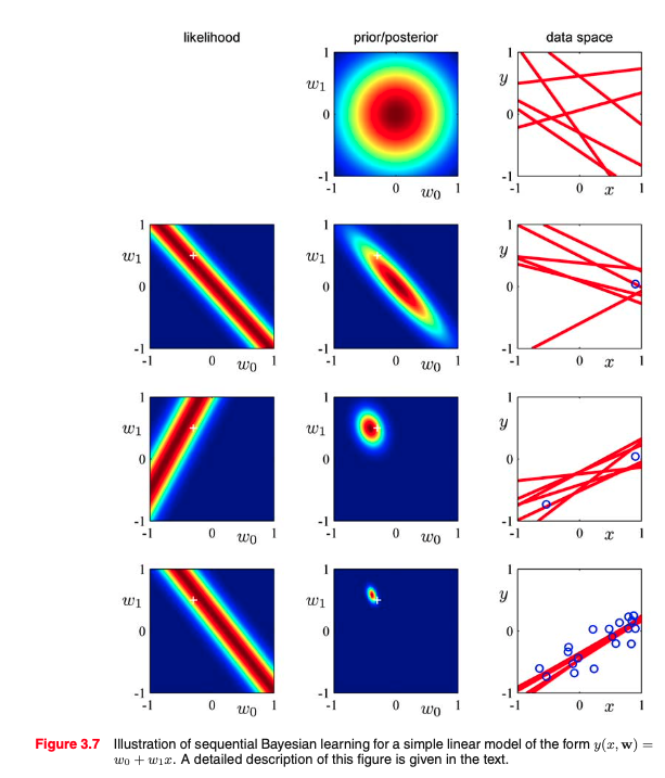
To go probabilistic, we have to make an assumption that each $y$ is generated linearly but with additive Gaussian Noise.

So

$$ y_i = \bmf{\theta}^T\mbf{x}_i + \epsilon$$

where $$ \epsilon = \mathcal{N}(0,\sigma^2)$$

• We observe $(\mbf{x}_i, y_i)$ but we do not know $\bmf{\theta}$ and the noise $\epsilon$.
• The noise changes from sample to sample but we know it is distributed as Gaussian.

Probabilistic Interpretation for Linear Regression

To go probabilistic, we have to make an assumption that each $y$ is generated linearly but with additive Gaussian Noise.

So

$$ \epsilon = y_i - \bmf{\theta}^T\mbf{x}_i \sim \mathcal{N}(0,\sigma^2)$$

• We observe $(\mbf{x}, y_i)$ but we do not know $\bmf{\theta}$ and the noise $\epsilon$.
• The noise changes from sample to sample but we know it is distributed as Gaussian.

What does the noise look like?

What does the noise look like?

Probabilistic Interpretation for Linear Regression

To go probabilistic, we have to make an assumption that each $y$ is generated linearly but with additive Gaussian Noise.

So

$$ \epsilon_i = y_i - \bmf{\theta}^T\mbf{x}_i \sim \mathcal{N}(0,\sigma^2)$$

which means the errors behave IID from a Normal Distribution.

$$ p\left(\epsilon_i\right)=\frac{1}{\sqrt{2 \pi} \sigma} \exp \left(-\frac{\epsilon_i^{2}}{2 \sigma^{2}}\right) $$

Probabilistic Interpretation for Linear Regression

We look at the conditional probability of $y$ given $\mbf{x}$ aka $p(y|\mbf{x}; \bmf{\theta})$:

$$ p\left(y_i \mid x_i ; \theta\right)=\frac{1}{\sqrt{2 \pi} \sigma} \exp \left(-\frac{\left(y_i-\theta^{T} x_i\right)^{2}}{2 \sigma^{2}}\right) $$

now is function of $y$ yet centered on $\theta^{T} x_i$: $$ y_i \mid x_i ; \theta \sim \mathcal{N}\left(\theta^{T} x_i, \sigma^{2}\right) $$

Estimate $\bmf{\theta}$ by Maximum Likelihood (MLE)

For a single training point:

$$ p\left(y_i \mid x_i ; \theta\right) \doteq L(\bmf{\theta};\mbf{x}_i,y_i) = \frac{1}{\sqrt{2 \pi} \sigma} \exp \left(-\frac{\left(y_i-\theta^{T} x_i\right)^{2}}{2 \sigma^{2}}\right) $$

Estimate $\bmf{\theta}$ by Maximum Likelihood (MLE)

For multiple training point $\{\mbf{x}_i,y_i\}$, given IID assumptions on $\epsilon$ and thus $y|x$

$$ \begin{aligned} L(\theta) &=\prod_{i=1}^{n} p\left(y^{(i)} \mid x^{(i)} ; \theta\right) \\ &=\prod_{i=1}^{n} \frac{1}{\sqrt{2 \pi} \sigma} \exp \left(-\frac{\left(y^{(i)}-\theta^{T} x^{(i)}\right)^{2}}{2 \sigma^{2}}\right) \end{aligned} $$

Maximizing the Log Likelihood (MLE)

$$ \begin{aligned} \ell(\theta) &=\log L(\theta) \\ &=\log \prod_{i=1}^{n} \frac{1}{\sqrt{2 \pi} \sigma} \exp \left(-\frac{\left(y^{(i)}-\theta^{T} x^{(i)}\right)^{2}}{2 \sigma^{2}}\right) \\ &=\sum_{i=1}^{n} \log \frac{1}{\sqrt{2 \pi} \sigma} \exp \left(-\frac{\left(y^{(i)}-\theta^{T} x^{(i)}\right)^{2}}{2 \sigma^{2}}\right) \\ &=n \log \frac{1}{\sqrt{2 \pi} \sigma}-\frac{1}{\sigma^{2}} \cdot \frac{1}{2} \sum^{n}\left(y^{(i)}-\theta^{T} x^{(i)}\right)^{2} \end{aligned} $$

Maximizing the Log Likelihood (MLE) equals Minimizing the Squared Loss

(Under the assumption that the errors will have distributions as Gaussians)

$$\arg\max_{\bmf{\theta}} n \log \frac{1}{\sqrt{2 \pi} \sigma}-\frac{1}{\sigma^{2}} \cdot \frac{1}{2} \sum^{n}\left(y^{(i)}-\theta^{T} x^{(i)}\right)^{2} \rightarrow \arg\min_{\bmf{\theta}} \frac{1}{2} \sum_{i=1}^{n}\left(y^{(i)}-\theta^{T} x^{(i)}\right)^{2} $$

To summarize: Under the previous probabilistic assumptions on the data, least-squares regression corresponds to finding the maximum likelihood estimate of θ. This is thus one set of assumptions under which least-squares regression can be justified as a very natural method that’s just doing maximum likelihood estimation.

(Note however that the probabilistic assumptions are by no means necessary for least-squares to be a perfectly good and rational procedure, and there may—and indeed there are—other natural assumptions that can also be used to justify it.)

Let's assume we could not find a closed form solution but we know how to program plus a bit of calculus, can we still solve Linear Regression?

We cannot derive a closed form solution...

We need to minimize $$ \mathcal{J}(\mbf{\theta};\mbf{x},y)= \frac{1}{2} \sum_{i=1}^{n}\mathcal{L}\big(y_{i}, f_{\boldsymbol{\theta}}(\mbf{x}_i)\big)$$ so to find:

$$\mbf{\theta}^{\star} = \arg\min_{\mbf{\theta}} \mathcal{J}(\mbf{\theta};\mbf{x},y) $$

👋🏼 Closed Form Solution; 🤗 Iterative Methods

In general, if you can find a closed form solution, that is the best you can do.

So if your problem is as simple as inverting a linear system, please **invert a linear system and use pseudo-inverse if you need to!**

In case you cannot derive, we can use numerical, iterative methods

A very simple yet effective Iterative method is Gradient Descent

• This part that we explain now starts to be propaedeutic for Deep Learning.

%matplotlib inline
from sklearn import linear_model, datasets
from matplotlib import pyplot as plt
import numpy as np

n_samples = 100
size = 7

X, y, coef_gt = datasets.make_regression(
    n_samples=n_samples,
    n_features=1,
    n_informative=1,
    noise=20,
    coef=True,
    random_state=42,
)
fig = plt.figure(figsize=(size, size))
ax = fig.add_subplot()
# Linear Regression
bias = np.ones((X.shape[0], 1))
X = np.hstack((X, bias))
theta = np.linalg.inv(X.T@X)@X.T@y
# Now MeshGrid
x_interp = np.linspace(Xmin, Xmax, 100)
x_interp = x_interp.reshape(-1,1)
x_interp = np.c_[x_interp,np.ones_like(x_interp)]
y_interp = np.dot(theta, x_interp.T)
ax.scatter(x_interp[:,0], y_interp, alpha=0.7, marker='.')
ax.scatter(X[..., 0], y, c='red', marker='o')
ax.set_xlabel('$x$');
ax.set_ylabel('$y$');

%matplotlib inline
from sklearn import linear_model, datasets
from matplotlib import pyplot as plt
import numpy as np

n_samples = 100
size = 7

X, y, coef_gt = datasets.make_regression(
    n_samples=n_samples,
    n_features=1,
    n_informative=1,
    noise=20,
    coef=True,
    random_state=42,
)
fig = plt.figure(figsize=(size, size))
ax = fig.add_subplot()
# Linear Regression
bias = np.ones((X.shape[0], 1))
X = np.hstack((X, bias))
theta = np.linalg.inv(X.T@X)@X.T@y
# Now MeshGrid
x_interp = np.linspace(Xmin, Xmax, 100)
x_interp = x_interp.reshape(-1,1)
x_interp = np.c_[x_interp,np.ones_like(x_interp)]
y_interp = np.dot(theta, x_interp.T)
ax.scatter(x_interp[:,0], y_interp, alpha=0.7, marker='.')
ax.scatter(X[..., 0], y, c='red', marker='o')
ax.set_xlabel('$x$');
ax.set_ylabel('$y$');

fig = plt.figure(figsize=(size-1, size-1))
plt.rcParams['axes.grid'] = False
plt.contourf(xxt, yyt, losses, levels=50, cmap='jet');
plt.colorbar()
plt.scatter(coef_gt,0,color='red',marker='o',s=50)
plt.axis('scaled')
plt.xlabel('$theta_1$')
plt.ylabel('$theta_2$');

Ready for an awesome demo?

## Implementation of Gradient Descent for Logistic Regression

import time
%matplotlib notebook


def get_diff(X, theta, y):
    return X@theta - y[..., np.newaxis]


def get_loss(diff): 
    return 0.5*np.dot(diff.T, diff)


def plot_line(plot3, theta):
    x_interp = np.linspace(Xmin, Xmax, 100)
    x_interp = x_interp.reshape(-1, 1)
    x_interp = np.c_[x_interp, np.ones_like(x_interp)]
    y_interp = np.dot(x_interp, theta)
    if plot3:
        plot3.set_xdata(x_interp[:, 0])
        plot3.set_ydata(y_interp)
    else:
        return x_interp, y_interp


plt.ion()
figure, (axes_1, axes_2) = plt.subplots(2, 2, figsize=(9, 9))
plt.rcParams['axes.grid'] = False
ax0, ax1 = axes_1
ax2, ax3 = axes_2
ax0.contourf(xxt, yyt, losses, levels=50, cmap='jet')
ax0.scatter(coef_gt, 0, color='red', marker='o', s=50)
ax0.set_xlabel('$theta_1$',fontsize=18)
ax0.set_ylabel('$theta_2$',fontsize=18)
ax1.set_ylabel('$loss$',fontsize=18)
ax1.set_xlabel('$iter$',fontsize=18)
ax1.set(xlim=(0, 100), ylim=(0, 1.28e6))
ax2.scatter(X[..., 0], y, c='red', marker='o')
ax2.set_xlabel('$x$',fontsize=18)
ax2.set_ylabel('$y$',fontsize=18)
ax3.set_ylabel('$Grad. Norm.$',fontsize=18)
ax3.set_xlabel('$iter$',fontsize=18)
ax3.set(xlim=(0, 100), ylim=(0, 20000))

theta_curr = np.array([[-100, -100]]).T
losses_track = [get_loss(get_diff(X, theta_curr, y))]
grad_norm_track = [1000]

theta_track = np.array(theta_curr)
lr = 1e-3
loss_tol = 10

plot1, = ax0.plot(*theta_curr, color='violet',
                  marker='.', markersize=5, linestyle='-')
plot2, = ax1.plot(*losses_track, color='blue',
                  marker='.', markersize=10, linestyle='--')
xi, yi = plot_line(None, theta_curr)
plot3a,plot3b = ax2.plot(xi, yi, color='blue', marker='.',
                  markersize=3, linestyle='--')
plot4, = ax3.plot(1000, color='blue',
                  marker='.', markersize=10, linestyle='--')
while True:
    diff = get_diff(X, theta_curr, y)
    grad = (diff * X).sum(axis=0, keepdims=True).T
    theta_curr = theta_curr - lr*grad
    theta_track = np.append(theta_track, theta_curr, axis=1)
    diff = get_diff(X, theta_curr, y)
    losses_track.append(get_loss(diff))
    grad_norm_track.append(np.linalg.norm(grad,2))
    if abs(losses_track[-2]-losses_track[-1]) < loss_tol:
        break
    plot1.set_xdata(theta_track[0, :])
    plot1.set_ydata(theta_track[1, :])
    plot2.set_xdata(range(len(losses_track)))
    plot2.set_ydata(losses_track)
    plot4.set_xdata(range(len(grad_norm_track[1:])))
    plot4.set_ydata(grad_norm_track[1:])
    plot_line(plot3a, theta_curr)
    plot_line(plot3b, theta_curr)
    figure.canvas.draw()
    figure.canvas.flush_events()
    time.sleep(0.1)
print(*theta_curr)
plt.show()

[46.09610615] [1.80913084]

Gradient Descent (GD)

$$ \mathcal{J}(\mbf{\theta};\mbf{x},y)= \frac{1}{2} \sum_{i=1}^{n}\mathcal{L}\big(y_{i}, f_{\boldsymbol{\theta}}(\mbf{x}_i)\big)$$

where

$$\mathcal{L}\big(y, f_{\boldsymbol{\theta}}(\mbf{x})\big) = \big(f_{\boldsymbol{\theta}}(\mbf{x}) - y \big)^2 $$$$\bmf{\hat{\theta}} = \arg \min_{\bmf{\theta}} \frac{1}{2} \sum_{i=1}^n \big(f_{\boldsymbol{\theta}}(\mbf{x}_i) - y_i \big)^2 $$

Analysis

The function $\mathcal{J}(\mbf{\theta};\mbf{x},y)$ is a convex quadratic function. The Hessian of $\mathcal{J}(\mbf{\theta};\mbf{x},y)$ at any vector $\theta$ is the positive definite matrix $\mbf{X}^T\mbf{X}$. Since $\mathcal{J}$ is lower bounded and grows at infinity, there is a minimum.

• if $\operatorname{rank}({\mbf{X}}) =\min\{d,n\}$ then $\mbf{X}^T\mbf{X}$ is strictly positive definite. In this case the error function $\mathcal{J}$ is strictly convex, so the minimum is unique (Ball Shape)
• if $\operatorname{rank}({\mbf{X}}) < \min\{d,n\}$ then $\mathcal{J}$ is not strictly convex and the minimum is not unique

plt.rcParams['axes.grid'] = False
fig = plt.figure(figsize=(4, 4))
ax = fig.add_subplot(111, projection='3d')
ax.plot_surface(xxt, yyt, losses, cmap='jet')
ax.set_xlabel('$theta_1$')
ax.set_zlabel('$J$')
ax.set_ylabel('$theta_2$');

Gradient Descent Algorithm as an Iterative Method

**Idea: make a little step so that locally after each step the cost is lower than before**
Input: Training set $\{\mbf{x}_i,y_i\}$, learning rate $\gamma$, a small value in $\{0.1,\ldots,\texttt{1e-6}\}$.

1. Initialization - Very Important if the function is not strictly convex

$$\bmf{\theta} \doteq \mbf{0}^T$$

Set it to all zeros or random initialization from a distribution. |

1. Repeat until convergence:
   • Compute the gradient of the loss wrt the parameters $\bmf{\theta}$ given all the training set
   • Take a small step in the opposite direction of steepest ascent (so steepest descent).
     
     $$\bmf{\theta} \leftarrow \bmf{\theta} -\gamma \bmf{\nabla}_{\bmf{\theta}}\mathcal{J}(\mbf{\theta};\mbf{x},y)$$
2. When convergence is reached, your final estimate is in $\bmf{\theta}$

Convergence

$$\big\{\bmf{\theta}_{t=0},\bmf{\theta}_{t=1}, \ldots, \bmf{\theta}_{t=100} \big\}$$

0) Always: validation loss/metric (early stopping) (required)

1) No significant decrease in the loss function (preferred)

$$\mid \mathcal{J}(\mbf{\theta};\mbf{x},y)_{t} - \mathcal{J}(\mbf{\theta};\mbf{x},y)_{t-1} \mid $$

1) No variations in the parameters

$$\mid\mid \mbf{\theta}_{t} - \mbf{\theta}_{t-1} \mid\mid $$

2) Gradient Norm goes to zero

$$\mid\mid \bmf{\nabla}_{\bmf{\theta}}\mathcal{J}(\mbf{\theta};\mbf{x},y) \mid\mid \rightarrow 0 $$

Gradient Descent on Linear Regression

1. Initialization $$\bmf{\theta} \sim \texttt{random}~~\text{or zero}$$
2. $$\bmf{\theta} \leftarrow \bmf{\theta} -\gamma \bmf{\nabla}_{\bmf{\theta}}\mathcal{J}(\mbf{\theta};\mbf{x},y)$$

$$\bmf{\theta} \leftarrow \bmf{\theta} -\gamma \bmf{\nabla}_{\bmf{\theta}} \frac{1}{2} \sum_{i=1}^n \big(\bmf{\theta}^T\mbf{x} - y \big)^2 $$$$\bmf{\theta} \leftarrow \bmf{\theta} -\gamma \frac{1}{2} \sum_{i=1}^n \big(2\bmf{\theta}^T\mbf{x}\mbf{x} - 2y\mbf{x} \big) $$$$\bmf{\theta} \leftarrow \bmf{\theta} -\gamma \sum_{i=1}^n \big(\bmf{\theta}^T\mbf{x}_i- y_i\big)\mbf{x}_i$$

Dimension Check

Summing up over ${\mbf{x}_i \in \mathbb{R}^d}$ scaled by the difference between the prediction and ground-truth

$$\bmf{\theta} \leftarrow \bmf{\theta} -\gamma \sum_{i=1}^n \big(\underbrace{\bmf{\theta}^T\mbf{x}_i- y_i\big)}_{\text{scalar}}\underbrace{\mbf{x}_i}_{\mathbb{R}^d}$$

Stochastic Gradient Descent (SGD)

Problem of GD: What happens if $n \mapsto \infty$.

To make a small step we have to go through ALL the training samples. Optimization could be slow for large $n$.

Idea: make an update for each single training sample selected randomly

$$\bmf{\theta} \leftarrow \bmf{\theta} -\gamma \big(\underbrace{\bmf{\theta}^T\mbf{x}_i- y_i\big)}_{\text{scalar}}\underbrace{\mbf{x}_i}_{\mathbb{R}^d} \qquad \text{where} \qquad i\sim \mathcal{U}(0,n)$$

Many Variations of SGD

Let's see the dynamic of SGD!

Another demo

# Implementation of Stochastic Gradient Descent for Logistic Regression

import time
%matplotlib notebook


def get_diff(X, theta, y):
    return X@theta - y[..., np.newaxis]


def get_loss(diff):
    return 0.5*np.dot(diff.T, diff)


def plot_line(plot3, theta):
    x_interp = np.linspace(Xmin, Xmax, 100)
    x_interp = x_interp.reshape(-1, 1)
    x_interp = np.c_[x_interp, np.ones_like(x_interp)]
    y_interp = np.dot(x_interp, theta)
    if plot3:
        plot3.set_xdata(x_interp[:, 0])
        plot3.set_ydata(y_interp)
    else:
        return x_interp, y_interp


plt.ion()
figure, (axes_1, axes_2) = plt.subplots(2, 2, figsize=(7, 7))
plt.rcParams['axes.grid'] = False
ax0, ax1 = axes_1
ax2, ax3 = axes_2
ax0.contourf(xxt, yyt, losses, levels=50, cmap='jet')
ax0.scatter(coef_gt, 0, color='red', marker='o', s=50)
ax0.set_xlabel('$theta_1$', fontsize=18)
ax0.set_ylabel('$theta_2$', fontsize=18)
ax1.set_ylabel('$loss$', fontsize=18)
ax1.set_xlabel('$iter$', fontsize=18)
ax1.set(xlim=(0, 100), ylim=(0, 1.28e6))
ax2.scatter(X[..., 0], y, c='red', marker='o')
ax2.set_xlabel('$x$', fontsize=18)
ax2.set_ylabel('$y$', fontsize=18)
ax3.set_ylabel('$Grad. Norm.$', fontsize=18)
ax3.set_xlabel('$iter$', fontsize=18)
ax3.set(xlim=(0, 100), ylim=(0, 300))

theta_curr = np.array([[-100, -100]]).T
losses_track = [get_loss(get_diff(X, theta_curr, y))]
grad_norm_track = [1000]

theta_track = np.array(theta_curr)
lr = 1e-1
loss_tol = 10
np.random.seed(42)

plot1, = ax0.plot(*theta_curr, color='violet',
                  marker='.', markersize=5, linestyle='-')
plot2, = ax1.plot(*losses_track, color='blue',
                  marker='.', markersize=10, linestyle='--')
xi, yi = plot_line(None, theta_curr)
plot3a, plot3b = ax2.plot(xi, yi, color='blue', marker='.',
                          markersize=3, linestyle='--')
plot4, = ax3.plot(1000, color='blue',
                  marker='.', markersize=10, linestyle='--')
while True:
    diff = get_diff(X, theta_curr, y)
    # STOCHASTIC PART ########################
    idx_sampled = np.random.randint(n_samples)
    grad = (diff * X)[idx_sampled, :].T.reshape(-1, 1)
    ##############################
    theta_curr = theta_curr - lr*grad
    theta_track = np.append(theta_track, theta_curr, axis=1)
    diff = get_diff(X, theta_curr, y)
    losses_track.append(get_loss(diff))
    grad_norm_track.append(np.linalg.norm(grad, 2))
    if abs(losses_track[-2]-losses_track[-1]) < loss_tol:
        break
    plot1.set_xdata(theta_track[0, :])
    plot1.set_ydata(theta_track[1, :])
    plot2.set_xdata(range(len(losses_track)))
    plot2.set_ydata(losses_track)
    plot4.set_xdata(range(len(grad_norm_track[1:])))
    plot4.set_ydata(grad_norm_track[1:])
    plot_line(plot3a, theta_curr)
    plot_line(plot3b, theta_curr)
    figure.canvas.draw()
    figure.canvas.flush_events()
    time.sleep(0.1)
print(*theta_curr)
plt.show()

[42.27801342] [-3.01691851]

Stochastic Gradient Descent (SGD): lots of Variations

• Zig-Zag "Noisy" Trajectory of SGD
• Converge to a $\gamma$-ball of the solution of GD
• Increases the iterations wrt GD
• Each iteration is so fast that the speed of SGD is much higher than GD for large training set $n$.

Notable Variations for Deep Learning

• SGD on mini-batches (a trade-off between SGD and GD)
• SGD with momentum (memory of previous state)

Many Variations of SGD

Machine Learning

---

7. Polynomial Regression, Feature Maps, Ridge Regression

Prof. Iacopo Masi - Computer Science Department, Sapienza University of Rome

Recap

We go back to your loved 🥰 Linear Algebra

Supervised, Parametric Models

1) Ordinary Linear Regression with Least Squares

2) Probabilistic Interpretation

3) Gradient Descent "Family"

Gradient Descent and [Stochastic] GD

1. Initialization - Very Important if the function is not strictly convex $$\bmf{\theta} \doteq \mbf{0}^T$$ Set it to all zeros or random initialization from a distribution.
2. Repeat until convergence:
   • Compute the gradient of the loss wrt the parameters $\bmf{\theta}$ given all the training set
   • Take a small step in the opposite direction of steepest ascent (so steepest descent).
     
     $$\bmf{\theta} \leftarrow \bmf{\theta} -\gamma \bmf{\nabla}_{\bmf{\theta}}\mathcal{J}(\mbf{\theta};\mbf{x},y)$$
3. When convergence is reached, your final estimate is in $\bmf{\theta}$

Many Variations of SGD

GD

$$\bmf{\theta} \leftarrow \bmf{\theta} -\gamma \sum_{i=1}^n \big(\underbrace{\bmf{\theta}^T\mbf{x}_i- y_i\big)}_{\text{scalar}}\underbrace{\mbf{x}_i}_{\mathbb{R}^d}$$

SGD

$$\bmf{\theta} \leftarrow \bmf{\theta} -\gamma \big(\underbrace{\bmf{\theta}^T\mbf{x}_i- y_i\big)}_{\text{scalar}}\underbrace{\mbf{x}_i}_{\mathbb{R}^d} \qquad \text{where}~ i\sim \mathcal{U}(0,n)$$

Maximizing the Log Likelihood (MLE) equals Minimizing the Squared Loss

(Under the assumption that the errors will have distribution as Gaussians)

$$\arg\max_{\bmf{\theta}} n \log \frac{1}{\sqrt{2 \pi} \sigma}-\frac{1}{\sigma^{2}} \cdot \frac{1}{2} \sum^{n}\left(y^{(i)}-\theta^{T} x^{(i)}\right)^{2} \rightarrow \arg\min_{\bmf{\theta}} \frac{1}{2} \sum_{i=1}^{n}\left(y^{(i)}-\theta^{T} x^{(i)}\right)^{2} $$

To summarize: Under the previous probabilistic assumptions on the data, least-squares regression corresponds to finding the maximum likelihood estimate of θ. This is thus one set of assumptions under which least-squares regression can be justified as a very natural method that’s just doing maximum likelihood estimation.

(Note however that the probabilistic assumptions are by no means necessary for least-squares to be a perfectly good and rational procedure, and there may—and indeed there are—other natural assumptions that can also be used to justify it.)

Today

Make Linear Regression... Non-Linear

Polynomial Regression with Basis Functions (Feature Map)

From Feature Maps to Kernel Methods

This lecture material is taken from

• Mostly from Bishop - Chapter 3 page 137
• Stanford notes
• Tibshirani - Chapter 4 page 43
• Sklearn Polynomial Regression

Linear Hypothesis

We assume relations $f \longleftrightarrow y$ is linear We know $D = \{\mbf{x}_i,y_i\}_{i=1}^n$ and we want to find ${\boldsymbol{\theta}}\doteq (\theta_0,\ldots,\theta_d)$

$$ f_{\boldsymbol{\theta}}(\mbf{x}) = \theta_0+ \theta_1\cdot x_1 + \theta_2\cdot x_2 + \ldots + \theta_d\cdot x_d$$

So ${\boldsymbol{\theta}}\doteq (\theta_0,\ldots,\theta_d) \in \mathbb{R}^{d+1}$.

$$ f_{\boldsymbol{\theta}}(\mbf{x}) = \big(\sum_{i=1}^d\theta_i\cdot x_i\big) + \theta_0$$

Trick for Notation Compactness

We can augment each feature to have a bias (intercept term) set to $1$ so that $\mbf{x} \doteq [1,\mbf{x}]$.

Doing so $\mbf{x} \in \mathbb{R}^{d+1}$

$$ f_{\boldsymbol{\theta}}(\mbf{x}) = \theta_0\cdot \underbrace{x_0}_{\text{always}~1} + \theta_1\cdot x_1 + \theta_2\cdot x_2 + \ldots + \theta_d\cdot x_d$$

So ${\boldsymbol{\theta}}\doteq (\theta_0,\ldots,\theta_d) \in \mathbb{R}^{d+1}$.

$$ f_{\boldsymbol{\theta}}(\mbf{x}) = \sum_{i=0}^d\theta_i\cdot x_i = \bmf{\theta}^T\mbf{x} $$

Linear Function of parameters $\bmf{\theta}$ and input $\mbf{x}$

With $\mbf{x} = [1,x_1,\ldots,x_d]$ and $\mbf{\theta} = [\theta_0,\theta_1,\ldots,\theta_d]$, we have:

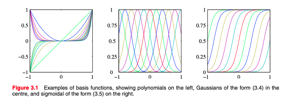
$$ f_{\boldsymbol{\theta}}(\mbf{x}) = \sum_{i=0}^d\theta_i\cdot x_i = \bmf{\theta}^T\mbf{x} $$

Does not capture non-linear relationships between $y$ and $\mbf{x}$

Interpreting Linear Regression with Basis Functions

We can have another dimensionality $m$ instead of $d$ by using Basis Functions $\bmf{\phi}(\mbf{x})$.

With $\bmf{\phi}(\mbf{x} = [1,\phi(x_1),\ldots,\phi(x_m)]$ and $\mbf{\theta} = [\theta_0,\theta_1,\ldots,\theta_m]$, we have:

$$ f_{\boldsymbol{\theta}}(\mbf{x}) = \sum_{i=0}^m\theta_i\cdot x_i = \bmf{\theta}^T\bmf{\phi}(\mbf{x}) $$

For Linear Regression:

• $m=d$, and
• the Basis Functions is : $\phi_m(\mbf{x}) = x_m$

What if..

• $m \neq d$, and
• the Basis Functions is : $\bmf{\phi}_m(\mbf{x}) \neq x_m$

then we do not have Linear Regression, and the settings impact the model

Think Basis Function as (Non-Linear) Transform or Feature Map

Let's consider the one dimensional case. We have already seen that we could change the feature $x$ to add the bias term $\mbf{x}\doteq [x,1]$

\begin{align} \mbf{x} &= \begin{bmatrix} x \\ 1 \end{bmatrix} \rightarrow \quad \bmf{\phi}(\mbf{x}) &= \begin{bmatrix} x^2\\ x \\ 1 \end{bmatrix} \end{align}

So input dimension is $d=2$ then output dimension after $\bmf{\phi}(\cdot)$ is $m=3$.

In this case we used a second order polynomial to lift up the features $$\bmf{\phi}_m(\mbf{x}) = x^m$$

Basis Function as Non-Linear Transform

$$ f_{\boldsymbol{\theta}}(\mbf{x}) = \sum_{i=0}^m\theta_i\cdot \bmf{\phi}_i(x) = \bmf{\theta}^T\bmf{\phi}(\mbf{x}) = \theta_0 + \theta_1\cdot x +\theta_2\cdot x^2 $$

Important observation:

• This is still linear function of the parameters $\theta$, in fact we still take the dot product
• Though it is NON linear function of the features $x$

Two Observations

• This is still **linear function** of the parameters $\theta$
  • Good we can solve it with Linear Regression
• Though it is **NON linear function** of the features $x$
  • Even better, we capture non-linearity in the data

Polynomial Regression (Basis Function $\bmf{\phi}_m(\mbf{x}) = x^m$)

$$ f_{\boldsymbol{\theta}}(\mbf{x}) = \sum_{i=0}^m\theta_i\cdot \bmf{\phi}_i(x) = \bmf{\theta}^T\bmf{\phi}(\mbf{x}) = \theta_0 + \theta_1\cdot x +\theta_2\cdot x^2 $$

Important observation:

• This is still linear function of the parameters $\theta$, in fact we still take the dot product
• Though it is NON linear function of the features $x$
• $m$ is the degree of the Polynomial we consider
• $m$ the higher the degree, the more expressive is the model

Poly (Multi) Nomial (Names or Terms)

Non-Linear Data

Linear Hypothesis? 😬

Now let's solve it with Linear Regression (we assume no bias)

def solve_lstq(x, y):
    return np.linalg.inv(x.T@x)@x.T@y


plt.figure(figsize=(7, 7))
plt.scatter(x, y, c='red', marker='o', s=30)
plt.scatter(x_valid, y_valid, c='blue', marker='o', s=30)
theta = solve_lstq(x, y)
x_interp = np.linspace(-support_X*1.5, support_X*1.5, 100).reshape(-1, 1)
y_interp = np.dot(theta, x_interp.T)
plt.plot(x_interp[:, 0], y_interp.T, alpha=0.7, marker='.');

Let's check the training error (or fitting error)

err = np.power(y - np.dot(theta, x.T), 2).mean()

Numerically it seems pretty high!

16.42335475440827

Let's try a quadratic basis function

Let's consider the one dimensional case. We have already seen that we could change the feature $x$ to add the bias term $\mbf{x}\doteq [x,1]$

\begin{align} \mbf{x} &= \begin{bmatrix} x \\ 1 \end{bmatrix} \rightarrow \quad \bmf{\phi}(\mbf{x}) &= \begin{bmatrix} x^2\\ x \\ 1 \end{bmatrix} \end{align}

So input dimension is $d=1$ then output dimension after $\bmf{\phi}(\cdot)$ is $m=2$.

In this case we used a second order polynomial to lift up the features $$\bmf{\phi}_m(\mbf{x}) = x^m$$

The blessing of dimensionality

Let's consider the one dimensional case. We have already seen that we could change the feature $x$ to add the bias term $\mbf{x}\doteq [x,1]$

\begin{align} \mbf{x} &= \begin{bmatrix} x \\ 1 \end{bmatrix} \rightarrow \quad \bmf{\phi}(\mbf{x}) &= \begin{bmatrix} x^2\\ x \\ 1 \end{bmatrix} \end{align}

• In some sense this can be seen as opposite to the curse of dimensionality
• Though if you increase $m$ too much you may face curse of dimensionality again

Now we can still solve it with LS but $m=2$

We can have another dimensionality $m$ instead of $d$ by using Basis Functions $\bmf{\phi}(\mbf{x})$ .

With $\bmf{\phi}(\mbf{x} = [1,\phi(x_1),\ldots,\phi(x_m)]$ and $\mbf{\theta} = [\theta_0,\theta_1,\ldots,\theta_m]$, we have:

$$ f_{\boldsymbol{\theta}}(\mbf{x}) = \sum_{i=0}^m\theta_i\cdot \bmf{\phi}_i(x) = \bmf{\theta}^T\bmf{\phi}(\mbf{x}) $$

For Linear Regression:

• $m > d$, and
• the Basis Functions is : $\phi_m(\mbf{x}) = x^m$

%matplotlib inline
plt.figure(figsize=(7, 7))
plt.scatter(x, y, c='red',marker='o', s=30)
theta_q = solve_lstq(xq, y)
x_interp = np.linspace(-support_X*1.5, support_X*1.5, 100).reshape(-1, 1)
x_interp_q = np.c_[x_interp, x_interp**2]
y_interp_q = np.dot(theta_q.T, x_interp_q.T)
plt.plot(x_interp_q[:, 0], y_interp_q.T, alpha=0.7, marker='.');

Let's check the training error (or fitting error) again

err = np.power(y - np.dot(theta_q.T, xq.T), 2).mean()

Numerically it seems pretty high!

16.04107222204833

Now we can still solve it with LS but $m=3$

We can have another dimensionality $m$ instead of $d$ by using Basis Functions $\bmf{\phi}(\mbf{x})$ .

With $\bmf{\phi}(\mbf{x} = [1,\phi(x_1),\ldots,\phi(x_m)]$ and $\mbf{\theta} = [\theta_0,\theta_1,\ldots,\theta_m]$, we have:

$$ f_{\boldsymbol{\theta}}(\mbf{x}) = \sum_{i=0}^m\theta_i\cdot \bmf{\phi}_i(x) = \bmf{\theta}^T\bmf{\phi}(\mbf{x}) $$

For Linear Regression:

• $m > d$, and
• the Basis Functions is : $\phi_m(\mbf{x}) = x^m$

%matplotlib inline
xc = np.c_[x, x**2, x**3]  # make cubic features
plt.figure(figsize=(7, 7))
plt.scatter(x, y, c='red', marker='o', s=30);
theta_c = solve_lstq(xc,y)
x_interp_c = np.c_[x_interp, x_interp**2, x_interp**3]
y_interp_c = np.dot(theta_c.T, x_interp_c.T)
plt.plot(x_interp_c[:, 0], y_interp_c.T, alpha=0.7, marker='.');

Let's check the training error (or fitting error) again

err = np.power(y - np.dot(theta_c.T, xc.T), 2).mean()

Numerically it seems pretty high!

16.036146988841292

We can analyze what happens in function of $m$

We can have another dimensionality $m$ instead of $d$ by using Basis Functions $\bmf{\phi}(\mbf{x})$.

With $\bmf{\phi}(\mbf{x} = [1,\phi(x_1),\ldots,\phi(x_m)]$ and $\mbf{\theta} = [\theta_0,\theta_1,\ldots,\theta_m]$, we have:

$$ f_{\boldsymbol{\theta}}(\mbf{x}) = \sum_{i=0}^m\theta_i\cdot x_i = \bmf{\theta}^T\bmf{\phi}(\mbf{x}) $$

For Linear Regression:

• $m > d$, and
• the Basis Functions is : $\phi_m(\mbf{x}) = x^m$

from sklearn.preprocessing import PolynomialFeatures
from sklearn.linear_model import LinearRegression
from sklearn.pipeline import Pipeline
import numpy as np

errors = []
errors_valid = []
models = []
for m in range(1, 20):
    model = Pipeline([('poly', PolynomialFeatures(degree=m, include_bias=False, interaction_only=False)),
                      ('linear', LinearRegression(fit_intercept=False))])
    models.append(model)
    model = model.fit(x, y)
    x_interp = np.linspace(-support_X-offset_valid,
                           support_X+offset_valid, 100).reshape(-1, 1)
    y_interp = model.predict(x_interp)
    y_est = model.predict(x)
    errors.append(np.power(y - y_est, 2).mean())
    errors_valid.append(np.power(y_valid - model.predict(x_valid), 2).mean())
    # Draw
    plt.figure(figsize=(7, 7))
    plt.scatter(x, y, c='red', marker='o', s=30)
    plt.plot(x_interp, y_interp, alpha=0.7, marker='.')
    plt.ylim([-10, 10])

Now let's check both the errors in train and validation

fig, axes = plt.subplots(1,2, figsize=(20, 7))
axes[0].bar(range(1, 20), errors)
axes[1].bar(range(1, 20), errors_valid);
axes[1].set_ylim([0,200])
axes[0].set_ylim([0,200])
m_best = np.argmin(errors_valid)
print(f'M best (polynomial degree is) {m_best+1}')

M best (polynomial degree is) 3

# Draw
plt.figure(figsize=(7, 7))
plt.scatter(x, y, c='red', marker='.')
plt.scatter(x_valid, y_valid, c='blue', marker='.')
y_interp = models[m_best].predict(x_interp)
plt.plot(x_interp, y_interp, alpha=0.7, marker='.');
plt.ylim([-100,100]);

# Draw
plt.figure(figsize=(7, 7))
plt.scatter(x, y, c='red', marker='.')
plt.scatter(x_valid, y_valid, c='blue', marker='.')
y_interp = models[-1].predict(x_interp)
plt.plot(x_interp, y_interp, alpha=0.7, marker='.');
plt.ylim([-100,100]);

Over or Under Fitting

Problem of Polynomial Regression

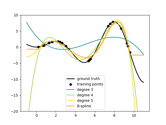
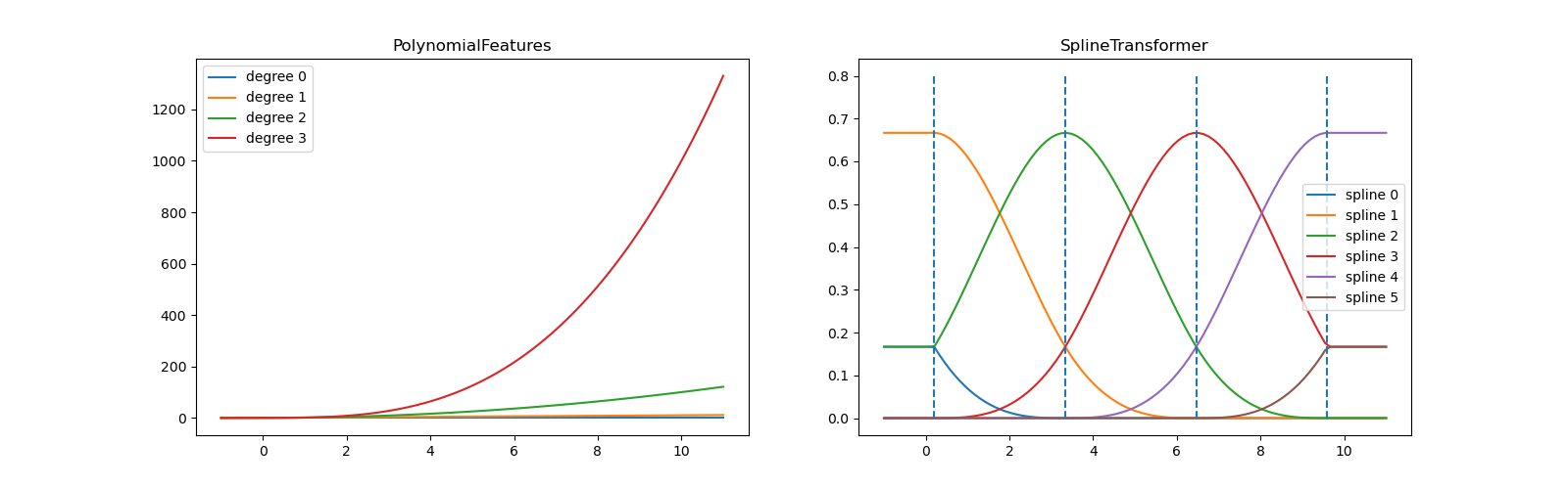
The basis function $\bmf{\phi}_m(\mbf{x}) = x^m$ is global wrt the domain of the feature $x$.

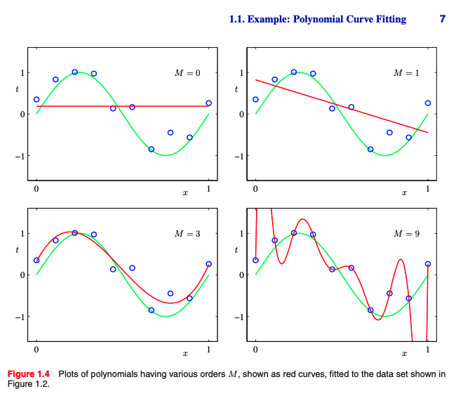
• The big limitation of polynomial basis functions is that they are global functions of the input variable, so that changes in one region of input space affect all other regions.

• This can be resolved by dividing the input space up into regions and fit a different polynomial in each region, leading to spline functions (that we do not cover).

Hint on Spline Functions

Other Basis Functions

Limitations of Basis Functions

Advantage: It is simple, and your problem stays convex and well behaved. (i.e. you can still use your original gradient descent code, just with the higher dimensional representation)

Disadvantage: $\phi(x)$ might be Very high dimensional.

X = PolynomialFeatures(interaction_only=True).fit_transform(X)

X_rand = np.array([[3, 7]], dtype=float)
print(f'Input Dimension {X_rand.shape}')
X_rand_poly = PolynomialFeatures(
    degree=2, interaction_only=False).fit_transform(X_rand)
print(f'Output Dimension {X_rand_poly.shape}')
print(X_rand[0, :], X_rand_poly[0, :], sep='\n')

Input Dimension (1, 2)
Output Dimension (1, 6)
[3. 7.]
[ 1.  3.  7.  9. 21. 49.]

%matplotlib inline
new_size = [PolynomialFeatures(degree=2, interaction_only=False).fit_transform(
    np.random.rand(1, d)).shape[1] for d in range(1, 50)]
plt.figure(figsize=(12,12))
plt.bar(range(1, 50), new_size);

Debug the Coefficients

Debug the Coefficients $\rightarrow$ Large Coefficients lead to overfit

Remedy for Large Coefficients: Weight Decay ($\ell_2$ Regularization)

We minimize the cost plus penalty term $$ \mathcal{J}(\mbf{\theta};\mbf{x},y)= \frac{1}{2} \sum_{i=1}^{n}\mathcal{L}\big(y_{i}, f_{\boldsymbol{\theta}}(\mbf{x}_i)\big) + \frac{\lambda}{2} \bmf{\theta}^T \bmf{\theta}= \frac{1}{2} \sum_{i=1}^{n}\mathcal{L}\big(y_{i}, f_{\boldsymbol{\theta}}(\mbf{x}_i)\big) + \frac{\lambda}{2} \vert\vert\bmf{\theta}\vert\vert_2^2 $$ so to find:

$$\mbf{\theta}^{\star} = \arg\min_{\mbf{\theta}} \mathcal{J}_{\text{data}}(\mbf{\theta};\mbf{x},y) +\lambda\mathcal{J}_{\text{reg.}}(\mbf{\theta}) $$

Still has a Closed Form Solution (Regularized Least Squares)

$$\bmf{\theta} = (\lambda \mbf{I} + \mbf{X}^T\mbf{X})^{-1} \mbf{X}^T\mbf{y}$$

Regularization allows complex models to be trained on data sets of limited size without severe over-fitting, essentially by limiting the effective model complexity

Linear Regression with Weight Decay ($\ell_2$ Regularization)

Consider the eigendecomposition of the symmetric Positive Semi Definite (PSD) matrix $\mbf{X}\mbf{X}^T$:

$$ X^{T} X= U \Sigma U^{T} =U \underbrace{\left[\begin{array}{ccc} \sigma_{1}^{2} & \ldots & 0 \\ \vdots & \ddots & \vdots \\ 0 & \ldots & \sigma_{d}^{2} \end{array}\right]}_{\operatorname{diag}\left(\sigma_{1}^{2}, \ldots, \sigma_{d}^{2}\right)} U^{T} $$

$\sigma_{1}^{2}, \ldots, \sigma_{d}^{2}$ are the eigenvalues and $ UU^{T} = Id$ (since $\Sigma$ is symmetric and square).

If $\mbf{X}$ and $\mbf{X}\mbf{X}^T$ are not full rank then some of $\sigma$ may be zeros.

Linear Regression with Weight Decay ($\ell_2$ Regularization)

This implies that if we regularized it, then the pseudo inverse is always invertible and has a unique solution since $\lambda > 0$:

$$ X^{T} X+\lambda I=U\left[\begin{array}{ccc} \sigma_{1}^{2}+\lambda & \ldots & 0 \\ \vdots & \ddots & \vdots \\ 0 & \ldots & \sigma_{d}^{2}+\lambda \end{array}\right] U^{T} $$

Linear Regression with Weight Decay ($\ell_2$ Regularization)

This implies that if we regularized it then the pseudo inverse is always invertible and has a unique solution since $\lambda > 0$:

$$ \left(X^{T} X+\lambda I\right)^{-1}=U\left[\begin{array}{ccc} \frac{1}{\sigma_{1}^{2}+\lambda} & \cdots & 0 \\ \vdots & \ddots & \vdots \\ 0 & \cdots & \frac{1}{\sigma_{d}^{2}+\lambda} \end{array}\right] U^{T} $$

Bias-Variance for Linear Reg. with Weight Decay ($\ell_2$ Regularization)

$$ \begin{aligned} \hat{\theta}_{n} &=\left(X^{T} X+\lambda I\right)^{-1} X^{T} \vec{y} \\ &=\left(X^{T} X+\lambda I\right)^{-1} X^{T}\left(X \theta^{*}+\vec{\epsilon}\right) \\ &=\left[\left(X^{T} X+\lambda I\right)^{-1} X^{T} X\right] \theta^{*}+\left[\left(X^{T} X+\lambda I\right)^{-1} X^{T}\right] \vec{\epsilon} \end{aligned} $$

$$ \begin{aligned} \mathbb{E}\left[\hat{\theta}_{n}\right]=& \mathbb{E}\left[\left[\left(X^{T} X+\lambda I\right)^{-1} X^{T} X\right] \theta^{*}+\left[\left(X^{T} X+\lambda I\right)^{-1} X^{T}\right] \vec{\epsilon}\right] \\ =& {\left[\left(X^{T} X+\lambda I\right)^{-1} X^{T} X\right] \theta^{*}+\left[\left(X^{T} X+\lambda I\right)^{-1} X^{T}\right] \mathbb{E}[\vec{\epsilon}] } \\ =& {\left[\left(X^{T} X+\lambda I\right)^{-1} X^{T} X\right] \theta^{*}+\left[\left(X^{T} X+\lambda I\right)^{-1} X^{T}\right] \overrightarrow{0} } \\ =& {\left[\left(X^{T} X+\lambda I\right)^{-1} X^{T} X\right] \theta^{*} } \\ =& U {\left[\begin{array}{ccc} \frac{1}{\sigma_{1}^{2}+\lambda} & \cdots & 0 \\ \vdots & \ddots & \vdots \\ 0 & \cdots & \frac{1}{\sigma_{d}^{2}+\lambda} \end{array}\right] U^{T} X^{T} X \theta^{*} } \\ =& U {\left[\begin{array}{ccc} \frac{1}{\sigma_{1}^{2}+\lambda} & \cdots & 0 \\ \vdots & \ddots & \vdots \\ 0 & \cdots & \frac{1}{\sigma_{d}^{2}+\lambda} \end{array}\right] \underbrace{U^{T} U}_{Id}\left[\begin{array}{ccc} \sigma_{1}^{2} & \ldots & 0 \\ \vdots & \ddots & \vdots \\ 0 & \ldots & \sigma_{d}^{2} \end{array}\right] U^{T} \theta^{*} } \\ =& U {\left[\begin{array}{ccc} \frac{1}{\sigma_{1}^{2}+\lambda} & \cdots & 0 \\ \vdots & \ddots & \vdots \\ 0 & \ldots & \frac{1}{\sigma_{d}^{2}+\lambda} \end{array}\right]\left[\begin{array}{ccc} \sigma_{1}^{2} & \ldots & 0 \\ \vdots & \ddots & \vdots \\ 0 & \ldots & \sigma_{d}^{2} \end{array}\right] U^{T} \theta^{*} } \\ =& U\left[\begin{array}{ccc} \frac{\sigma_{1}^{2}}{\sigma_{1}^{2}+\lambda} & \cdots & 0 \\ \vdots & \ddots & \vdots \\ 0 & \cdots & \frac{\sigma_{d}^{2}}{\sigma_{d}^{2}+\lambda} \end{array}\right] U^{T} \theta^{*} . \end{aligned} $$

Bias-Variance for Linear Reg. with Weight Decay ($\ell_2$ Regularization)

• From the above, we can make a few observations. First, when $\lambda=0$, we see that $\mathbb{E}[\theta_n] = \theta$. This implies that the standard linear regression estimator (without regularization) is Unbiased.
• The more regularization we add (i.e. larger $\lambda$), the smaller the eigenvalues will be, and hence the stronger the “shrinkage” towards 0. Thus it is biased towards zero.

Weight Decay arises from Bayesian Linear Regression

$$ \epsilon = y_i - \bmf{\theta}^T\mbf{x}_i \sim \mathcal{N}(0,\sigma^2)$$$$ \mbf{\theta} \sim \mathcal{N}(0,\bmf{\Theta}^2) \quad \texttt{prior on weights}$$

Unlike MLE, now there is a Gaussian prior on the weights; We solve it by doing Maximum A Posteriori (MAP)

Hint on Bayesian Linear Regression