Machine Learning

Machine Learning

---

6. Generative Models

Prof. Iacopo Masi - Computer Science Department, Sapienza University of Rome

Note: Most of the slides are taken from Applied Machine Learning (Cornell CS5785

All the credits go to the authors.

Generative vs Discriminative Models in Machine Learning

Learning from complex distributions is in common to vision/NLP (curse of dimensionality)

Vision: high-dimensional, continuous data

$$ p(\mbf{x} )$$

NLP: combinatorial/compositional problem of discrete symbols

$$ p(w_1, \ldots, w_t) $$

pot and enough deep secret rat thunder black industry answer death material angle crime probable nation debt organization spade acid soup reward free circle west forward board bone substance parcel south scissors move window hanging needle sticky pipe table old river attack design expert

Unknown density of the data

$p_{\text{data}(\bx)}$

Picture from [Yang-Song Blog](https://yang-song.net/blog/2021/score/)

Known data samples dataset

$\{\mbf{x}_i\} \sim p_{\text{data}(\bx)}$

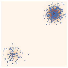
Picture from [Yang-Song Blog](https://yang-song.net/blog/2021/score/)

Generative vs Discriminative Models

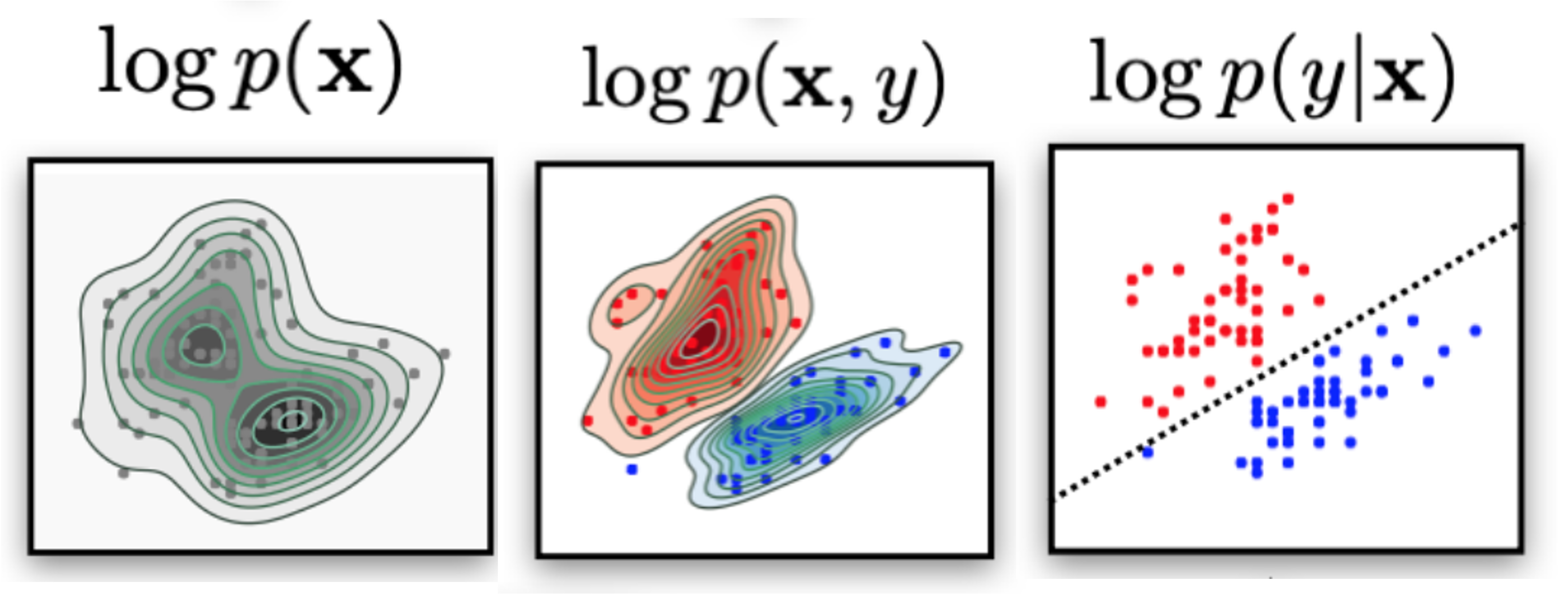
Generative models objective is to learn an approximation of the data density given the data samples (dataset):

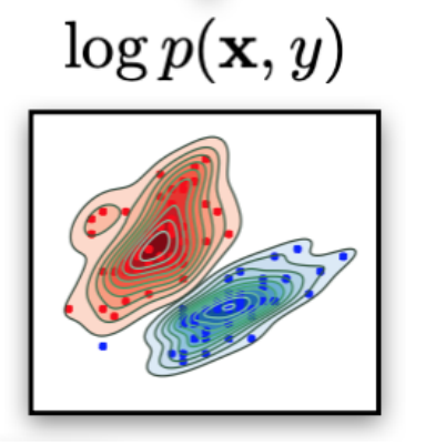
$$ p_{\text{data}}(\bx) \approx p_{\theta}(\bx)$$$$ p_{\text{data}}(\bx,y) \approx p_{\theta}(\bx,y)$$

Discriminative models objective is to learn a decision boundary to "separate" data samples to perform classification.

$$p(y == \text{class}~k | \bx)$$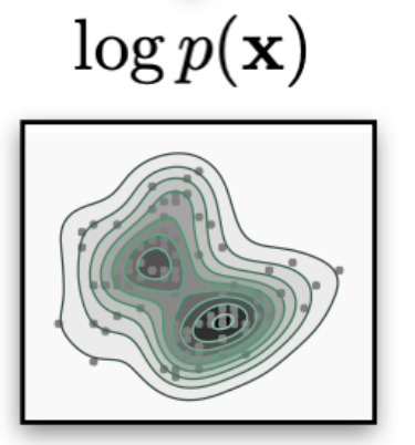

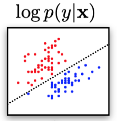
Generative

Discriminative

Generative and Discriminative are Connected

Think "classes" as latent factors in the data--the class label just "reveals" the latent factor. [There could be, there are others]. Think as "slicing the data density" using the latent factor ("coloring" the data density).

$$ p_{\theta}(\bx) = \sum_{y^{\prime}} p_{\theta}(\bx,y^{\prime}) \qquad \text{marginalization}$$

$$ p_{\theta}(\bx,y) = \underbrace{p(\bx|y)}_{\text{class-cond. density}}p(y) = \underbrace{p(y|\bx)}_{\text{discriminative}}p(\bx) \qquad \text{product rule}$$

Generative and Discriminative are Connected

$$\underbrace{p(y|\bx)}_{\text{discriminative}}p(\bx) = p_{\theta}(\bx,y) = \underbrace{p(\bx|y)}_{\text{generative}}p(y)$$

$$\underbrace{p(y|\bx)}_{\text{discriminative}} = \frac{p_{\theta}(\bx,y)}{p(\bx)} = \frac{p(\bx|y)p(y)}{p(\bx)} = \frac{p(\bx|y)p(y)}{\sum_{y^{\prime}} p(\bx|y)p(y^{\prime})}$$

From Generative go Discriminative

If you need to do just classification (and do not need probabilities):

$$\arg\max_{y^{\prime}} p(y^{\prime}|\bx)$$

Then you can:

1. Model/Estimate the class conditional data density $p(\bx|y)$ - think of the data density "restricted to one latent factor, a class".
2. Estimate how much do you think a latent factor (class) is probable $p(y)$
3. Classify as:

$$ \arg\max_{y^{\prime}} p(\bx|y^{\prime})p(y^{\prime}) \qquad \text{Given that} \quad p(y|\bx) \propto p(\bx|y)p(y)$$

Picture from [YOUR CLASSIFIER IS SECRETLY AN ENERGY BASED MODEL AND YOU SHOULD TREAT IT LIKE ONE](https://openreview.net/pdf?id=Hkxzx0NtDB)

The following slides are taken from Applied Machine Learning (Cornell CS5785

All the credits go to the authors.

Discriminative vs. Generative Models

Logistic regression is an example of a discriminative classifier. $$ P_\theta(y| x) = \left[ \begin{array}{c} P_\theta(y=0| x) \\ P_\theta(y=1| x) \\ \end{array} \right] $$

• It directly transforms $x$ into a score for each class $y$, e.g., via the formula $\sigma(\theta^\top x)$
• It can be interpreted as defining a conditional probability $P_\theta(y|x)$

Generative classifiers instead define distributions $P_\theta(x|y)$ and $P_\theta(y)$ over $x,y$.

Relation to text-to-image (TTI) models

• TTI models can also be written as $P(x|y)$, where $x$ is an image (millions of dimensions) and $y$ is a text description of it (many possibilities).
• This lecture: $x$ is a flower representation (4D), $y$ is a class (3 choices)

(Image source)

Generative Classifiers: Intuition

Imagine we have a dataset (e.g., flowers). We can fit a Gaussian to each class:

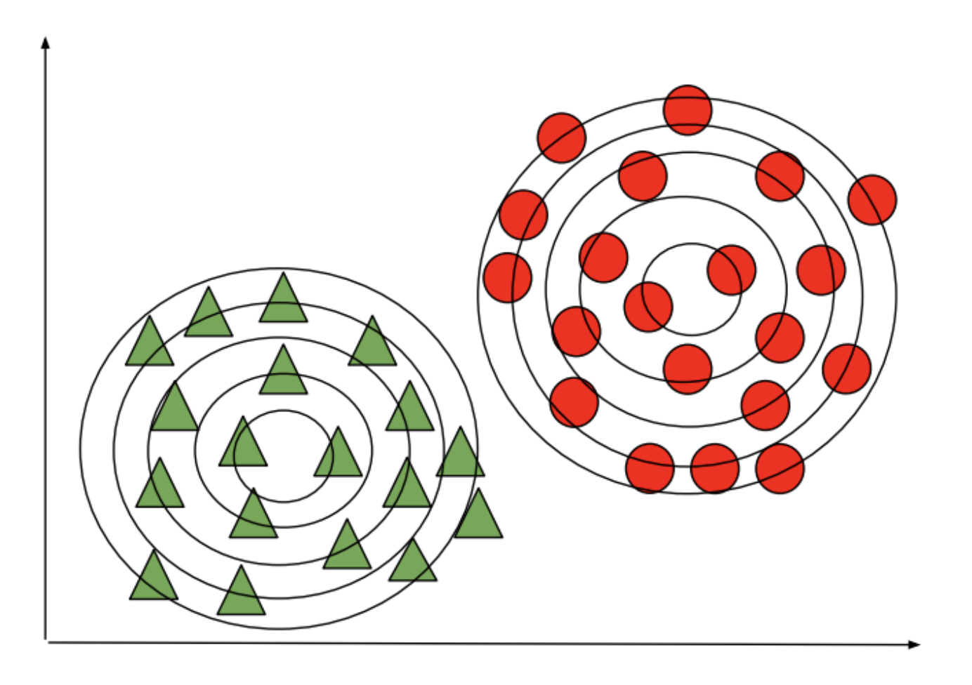
At test time, we predict the class of the Gaussian that is most likely to have generated the data.

Given a new flower $x'$, we would compare the probabilities of three models:

\begin{align*} P_\theta(x'|y=\text{0})P_\theta(y=\text{0}) \\ P_\theta(x'|y=\text{1})P_\theta(y=\text{1}) \\ P_\theta(x'|y=\text{2})P_\theta(y=\text{2}) \end{align*}

We output the class that's more likely to have generated $x'$.

Generative Classifiers: Details

Another approach to classification is to use generative models.

• A generative approach first builds a model of $x$ for each class: $$ P_\theta(x | y=k) \; \text{for each class $k$}.$$ $P_\theta(x | y=k)$ scores each $x$ according to how well it matches class $k$.

• A class probability $P_\theta(y=k)$ encoding our prior beliefs. These are often just the % of each class in the data.

In the context of flower classification (e.g., Setosa vs. non-Setosa), we would fit two models on a dataset of flower features $x$ with corresponding species labels $y$:

\begin{align*} P_\theta(x|y=\text{0}) && \text{and} && P_\theta(x|y=\text{1}) \end{align*}

• $P_\theta(x | y=1)$ scores each $x$ based on how much it looks like Iris Setosa.
• $P_\theta(x | y=0)$ scores each $x$ based on whether it looks like non-Setosa.

We also choose a prior $P(y)$.

Part 3: Gaussian Discriminant Analysis

Next, we will use GMMs as the basis for a new generative classification algorithm, Gaussian Discriminant Analysis (GDA).

The Parameters of a GMM

We need to learn the parameters of two sets of distributions:

• The distribution over classes is Categorical, denoted $\text{Categorical}(\phi_1, \phi_2, ..., \phi_K)$. Thus, $P_\theta(y=k) = \phi_k$.
• The conditional probability $P(x\mid y=k)$ of the data under class $k$ is a multivariate Gaussian $\mathcal{N}(x; \mu_k, \Sigma_k)$ with mean and covariance $\mu_k, \Sigma_k$.

Learning the Parameters $\mu_k, \Sigma_k$

• Consider the dataset of all the points $x$ for which $y=k$.
• Goal: learn the mean and variance $\theta_k=(\mu_k, \Sigma_k)$ of a Normal that generates $x$
• What is the maximum likelihood $\mu_k, \Sigma_k$ in this case? The formulation is:

$$\arg\max_{\theta_k} P_{\theta_k}(x|y=k)$$

• For Gaussians, these are the empirical means and covariances of each class. \begin{align*} \mu_k & = \frac{\sum_{i: y^{(i)} = k} x^{(i)}}{n_k} \\ \Sigma_k & = \frac{\sum_{i: y^{(i)} = k} (x^{(i)} - \mu_k)(x^{(i)} - \mu_k)^\top}{n_k} \\ \end{align*}

Learning the Parameters $\phi$

Next, consider learning $\vec \phi = (\phi_1, \phi_2, \ldots, \phi_K)$.

• We have $n$ datapoints. Each point has a label $k\in\{1,2,...,K\}$.
• Our model is a categorical and assigns a probability $\phi_k$ to each outcome $k\in\{1,2,...,K\}$.
• We want to infer $\phi_k$ assuming our dataset is sampled from the model.

What are the maximum likelihood $\phi_k$ that are most likely to have generated our data?

Intuitively, the maximum likelihood class probabilities $\phi$ should just be the class proportions that we see in the data. $$ \phi_k = \frac{n_k}{n}$$ for each $k$, where $n_k = |\{i : y^{(i)} = k\}|$ is the number of training targets with class $k$.

Thus, the optimal $\phi_k$ is just the proportion of data points with class $k$ in the training set!

Querying the Model

How do we ask the model for predictions? As discussed earlier, we can apply Bayes' rule: $$\arg\max_y P_\theta(y|x) = \arg\max_y P_\theta(x|y)P(y).$$ Thus, we can estimate the probability of $x$ and under each $P_\theta(x|y=k)P(y=k)$ and choose the class that explains the data best.

Algorithm: Gaussian Discriminant Analysis (GDA)

• Type: Supervised learning (multi-class classification)
• Model family: Mixtures of Gaussians.
• Objective function: Log-likelihood.
• Optimizer: Closed form solution.

Example: Iris Flower Classification

Let's see how this approach can be used in practice on the Iris dataset.

• We will learn the maximum likelihood GDA parameters
• We will compare the outputs to the true predictions.

Let's first start by computing the true parameters on our dataset.

# we can implement these formulas over the Iris dataset
d = 2 # number of features in our toy dataset
K = 3 # number of clases
n = X.shape[0] # size of the dataset

# these are the shapes of the parameters
mus = np.zeros([K,d])
Sigmas = np.zeros([K,d,d])
phis = np.zeros([K])

# we now compute the parameters
for k in range(3):
    X_k = X[iris_y == k]
    mus[k] = np.mean(X_k, axis=0)
    Sigmas[k] = np.cov(X_k.T)
    phis[k] = X_k.shape[0] / float(n)

We can look at the learned parameter values and compare them to the data

print('mus:', mus, '\nphis:', phis)

mus: [[5.01 3.43]
 [5.94 2.77]
 [6.59 2.97]] 
phis: [0.33 0.33 0.33]

plt.scatter(X[:, 0], X[:, 1], c=Y, edgecolors='k', cmap=plt.cm.Paired, s=50);
plt.xlabel('Sepal length'); plt.ylabel('Sepal width');

We can compute predictions using Bayes' rule.

# we can implement this in numpy
def gda_predictions(x, mus, Sigmas, phis):
    """This returns class assignments and p(y|x) under the GDA model.
    
    We compute \arg\max_y p(y|x) as \arg\max_y p(x|y)p(y)
    """
    # adjust shapes
    n, d = x.shape
    x = np.reshape(x, (1, n, d, 1))
    mus = np.reshape(mus, (K, 1, d, 1))
    Sigmas = np.reshape(Sigmas, (K, 1, d, d))    
    
    # compute probabilities
    py = np.tile(phis.reshape((K,1)), (1,n)).reshape([K,n,1,1])
    pxy = (
        np.sqrt(np.abs((2*np.pi)**d*np.linalg.det(Sigmas))).reshape((K,1,1,1)) 
        * -.5*np.exp(
            np.matmul(np.matmul((x-mus).transpose([0,1,3,2]), np.linalg.inv(Sigmas)), x-mus)
        )
    )
    pyx = pxy * py
    return pyx.argmax(axis=0).flatten(), pyx.reshape([K,n])

idx, pyx = gda_predictions(X, mus, Sigmas, phis)
print(idx)

[0 0 0 0 0 0 0 0 0 0 0 0 0 0 0 0 0 0 0 0 0 0 0 0 0 0 0 0 0 0 0 0 0 0 0 0 0
 0 0 0 0 1 0 0 0 0 0 0 0 0 2 2 2 1 2 1 2 1 2 1 1 1 1 1 1 2 1 1 1 1 1 1 2 1
 2 2 2 2 1 1 1 1 1 1 1 2 2 2 1 1 1 1 1 1 1 1 1 1 1 1 2 1 2 2 2 2 1 2 2 2 2
 2 2 1 1 2 2 2 2 1 2 1 2 1 2 2 1 1 2 2 2 2 2 1 1 2 2 2 1 2 2 2 1 2 2 2 2 2
 2 1]

We visualize the decision boundaries like we did earlier.

Z, pyx = gda_predictions(np.c_[xx.ravel(), yy.ravel()], mus, Sigmas, phis)
logpy = np.log(-1./3*pyx)

Z = Z.reshape(xx.shape)
contours = np.zeros([K, xx.shape[0], xx.shape[1]])
for k in range(K): contours[k] = logpy[k].reshape(xx.shape)
plt.pcolormesh(xx, yy, Z, cmap=plt.cm.Paired)
for k in range(K): plt.contour(xx, yy, contours[k], levels=np.logspace(0, 1, 1))

plt.scatter(X[:, 0], X[:, 1], c=iris_y, edgecolors='k', cmap=plt.cm.Paired)
plt.xlabel('Sepal length'); plt.ylabel('Sepal width');

Special Cases of GDA

Many important generative algorithms are special cases of GDA:

• Linear discriminant analysis (LDA): all the covariance matrices $\Sigma_k$ take the same value.
• Gaussian Naive Bayes: all the covariance matrices $\Sigma_k$ are diagonal.
• Quadratic discriminant analysis (QDA): another term for GDA (because the decision boundary is quadratic).

Part 4: Discriminative vs. Generative Classifiers

We conclude our lecture on generative classifiers by revisiting the question of how they compare to discriminative classifiers.

Linear Discriminant Analysis

When the covariances $\Sigma_k$ in GDA are equal, we have an algorithm called Linear Discriminant Analysis or LDA.

The probability of the data $x$ for each class is a multivariate Gaussian with the same covariance $\Sigma$. $$P_\theta(x|y=k) = \mathcal{N}(x ; \mu_k, \Sigma).$$

The probability over $y$ is Categorical: $P_\theta(y=k) = \phi_k$.

Let's try this algorithm on the Iris flower dataset.

We compute the model parameters similarly to how we did for GDA.

# we can implement these formulas over the Iris dataset
d = 2 # number of features in our toy dataset
K = 3 # number of clases
n = X.shape[0] # size of the dataset

# these are the shapes of the parameters
mus = np.zeros([K,d])
Sigmas = np.zeros([K,d,d])
phis = np.zeros([K])

# we now compute the parameters
for k in range(3):
    X_k = X[iris_y == k]
    mus[k] = np.mean(X_k, axis=0)
    Sigmas[k] = np.cov(X.T) # this is now X.T instead of X_k.T
    phis[k] = X_k.shape[0] / float(n)

# print out the means
print(mus)

[[5.01 3.43]
 [5.94 2.77]
 [6.59 2.97]]

We can compute predictions using Bayes' rule.

# we can implement this in numpy
def gda_predictions(x, mus, Sigmas, phis):
    """This returns class assignments and p(y|x) under the GDA model.
    
    We compute \arg\max_y p(y|x) as \arg\max_y p(x|y)p(y)
    """
    # adjust shapes
    n, d = x.shape
    x = np.reshape(x, (1, n, d, 1))
    mus = np.reshape(mus, (K, 1, d, 1))
    Sigmas = np.reshape(Sigmas, (K, 1, d, d))    
    
    # compute probabilities
    py = np.tile(phis.reshape((K,1)), (1,n)).reshape([K,n,1,1])
    pxy = (
        np.sqrt(np.abs((2*np.pi)**d*np.linalg.det(Sigmas))).reshape((K,1,1,1)) 
        * -.5*np.exp(
            np.matmul(np.matmul((x-mus).transpose([0,1,3,2]), np.linalg.inv(Sigmas)), x-mus)
        )
    )
    pyx = pxy * py
    return pyx.argmax(axis=0).flatten(), pyx.reshape([K,n])

idx, pyx = gda_predictions(X, mus, Sigmas, phis)
print(idx)

[0 0 0 0 0 0 0 0 0 0 0 0 0 0 0 0 0 0 0 0 0 0 0 0 0 0 0 0 0 0 0 0 0 0 0 0 0
 0 0 0 0 1 0 0 0 0 0 0 0 0 2 2 2 1 2 1 2 1 2 1 1 1 1 1 1 2 1 1 1 1 2 1 1 1
 2 2 2 2 1 1 1 1 1 1 1 2 2 1 1 1 1 1 1 1 1 1 1 1 1 1 2 1 2 2 2 2 1 2 1 2 2
 1 2 1 1 2 2 2 2 1 2 1 2 1 2 2 1 1 2 2 2 2 2 1 1 2 2 2 1 2 2 2 1 2 2 2 1 2
 2 1]

We visualize predictions like we did earlier.

Z, pyx = gda_predictions(np.c_[xx.ravel(), yy.ravel()], mus, Sigmas, phis)
logpy = np.log(-1./3*pyx)

Z = Z.reshape(xx.shape)
contours = np.zeros([K, xx.shape[0], xx.shape[1]])
for k in range(K):
    contours[k] = logpy[k].reshape(xx.shape)
plt.pcolormesh(xx, yy, Z, cmap=plt.cm.Paired)
for k in range(K):
    plt.contour(xx, yy, contours[k], levels=np.logspace(0, 1, 1))

plt.scatter(X[:, 0], X[:, 1], c=iris_y, edgecolors='k', cmap=plt.cm.Paired)
plt.xlabel('Sepal length'); plt.ylabel('Sepal width');

Linear Discriminant Analysis outputs decision boundaries that are linear, just like Logistic/Softmax Regression.

Softmax or Logistic regression also produce linear boundaries. In fact, both types of algorithms make use of the same model class.

Are the algorithms equivalent?

No! They assume the same model class $\mathcal{M}$, they use a different objective $J$ to select a model in $\mathcal{M}$.

nrow, ncol = 1, 2
fig, axs = plt.subplots(nrow, ncol, figsize=(6*ncol, 2*nrow))
axs[0].pcolormesh(xx, yy, Z, cmap=plt.cm.Paired); axs[0].set_title('LDA')
axs[1].pcolormesh(xx, yy, Z_lr, cmap=plt.cm.Paired); axs[1].set_title('Logistic Regression')

for ax in axs:
    ax.scatter(X[:, 0], X[:, 1], c=iris_y, edgecolors='k', cmap=plt.cm.Paired)
    ax.set_xlabel('Sepal length'); ax.set_ylabel('Sepal width')

LDA vs. Logistic Regression

What are the differences between LDA/NB and logistic regression?

• Bernoulli Naive Bayes or LDA assumes a logistic form for $P(y|x)$. But the converse is not true: logistic regression does not assume a NB or LDA model for $P(x,y)$.
• Generative models make stronger modeling assumptions. If these assumptions hold true, the generative models will perform better.
• But if they don't, logistic regression will be more robust to outliers and model misspecification, and achieve higher accuracy.

Discriminative Approaches

Discriminative algorithms are deservingly very popular.

• Most state-of-the-art algorithms for classification are discriminative (including neural nets, boosting, SVMs, etc.)
• They are often more accurate because they make fewer modeling assumptions.

Other Useful Features of Generative Models

Generative models can also do things that discriminative models can't do.

• Generation: we can sample $x \sim p(x|y)$ to generate new data (images, audio).
• Missing value imputation: if $x_j$ is missing, we infer it using $p(x|y)$.
• Outlier detection: we may detect via $p(x')$ if $x'$ is an outlier.
• Scalability: Simple formulas for maximum likelihood parameters.

Given a new $x'$, we would compare the probabilities of both models:

\begin{align*} P_\theta(x'|y=\text{0})P_\theta(y=\text{0}) && \text{vs.} && P_\theta(x'|y=\text{1})P_\theta(y=\text{1}) \end{align*}

We output the class that's more likely to have generated $x'$.

Naive Bayes

Part 1: Text Classification

We will now do a quick detour to talk about an important application area of machine learning: text classification.

Afterwards, we will see how text classification motivates new classification algorithms.

Text Classification

An interesting instance of a classification problem is classifying text.

• Many applications: spam filtering, fraud detection, medical record classification.
• Inputs $x$ are sequences of words of an arbitrary length.
• Limitation: Our algorithms take as input column vectors of a fixed dimension.

What do we do?

Bag of Words Representations

A widely-used approach to representing text documents is called "bag of words".

We start by defining a vocabulary $V$ containing all the possible words we are interested in, e.g.: $$ V = \{\text{church}, \text{doctor}, \text{fervently}, \text{purple}, \text{slow}, ...\} $$

A bag of words representation of a document $x$ is a function $\phi(x) \to \{0,1\}^{|V|}$ that outputs a feature vector $$ \phi(x) = \left( \begin{array}{c} 0 \\ 1 \\ 0 \\ \vdots \\ 1 \\ \vdots \\ \end{array} \right) \begin{array}{l} \;\text{church} \\ \;\text{doctor} \\ \;\text{fervently} \\ \vdots \\ \;\text{purple} \\ \vdots \\ \end{array} $$ of dimension $V$. The $j$-th component $\phi(x)_j$ equals $1$ if $x$ contains the $j$-th word in $V$ and $0$ otherwise.

Classification Dataset: Twenty Newsgroups

To illustrate the text classification problem, we will use a popular dataset called 20-newsgroups.

• It contains ~20,000 documents collected approximately evenly from 20 different online newsgroups.
• Each newgroup covers a different topic such as medicine, computer graphics, or religion.
• This dataset is often used to benchmark text classification and other types of algorithms.

Let's load this dataset.

#https://scikit-learn.org/stable/tutorial/text_analytics/working_with_text_data.html
    
from IPython.display import Markdown, display
import numpy as np; np.set_printoptions(precision=2)
import pandas as pd; pd.options.display.float_format = "{:,.2f}".format
from sklearn.datasets import fetch_20newsgroups

# for this lecture, we will restrict our attention to just 4 different newsgroups:
categories = ['alt.atheism', 'soc.religion.christian', 'comp.graphics', 'sci.med']

# load the dataset
twenty_train = fetch_20newsgroups(subset='train', categories=categories, shuffle=True, random_state=42)

# print some information on it
Markdown(twenty_train.DESCR[:1088])

.. _20newsgroups_dataset:

The 20 newsgroups text dataset

The 20 newsgroups dataset comprises around 18000 newsgroups posts on 20 topics split in two subsets: one for training (or development) and the other one for testing (or for performance evaluation). The split between the train and test set is based upon a messages posted before and after a specific date.

This module contains two loaders. The first one, :func:sklearn.datasets.fetch_20newsgroups, returns a list of the raw texts that can be fed to text feature extractors such as :class:~sklearn.feature_extraction.text.CountVectorizer with custom parameters so as to extract feature vectors. The second one, :func:sklearn.datasets.fetch_20newsgroups_vectorized, returns ready-to-use features, i.e., it is not necessary to use a feature extractor.

Data Set Characteristics:

=================   ==========
Classes                     20
Samples total            18846
Dimensionality               1
Features                  text
=================   ==========

# The set of targets in this dataset are the newgroup topics:
twenty_train.target_names

['alt.atheism', 'comp.graphics', 'sci.med', 'soc.religion.christian']

# Let's examine one data point
print(twenty_train.data[3])

From: s0612596@let.rug.nl (M.M. Zwart)
Subject: catholic church poland
Organization: Faculteit der Letteren, Rijksuniversiteit Groningen, NL
Lines: 10

Hello,

I'm writing a paper on the role of the catholic church in Poland after 1989. 
Can anyone tell me more about this, or fill me in on recent books/articles(
in english, german or french). Most important for me is the role of the 
church concerning the abortion-law, religious education at schools,
birth-control and the relation church-state(government). Thanx,

                                                 Masja,
"M.M.Zwart"<s0612596@let.rug.nl>

Let's see an example of Bag-of-Words on 20-newsgroups.

We start by computing these features using the sklearn library.

from sklearn.feature_extraction.text import CountVectorizer

# vectorize the training set
count_vect = CountVectorizer(binary=True)
X_train = count_vect.fit_transform(twenty_train.data)
X_train.shape

(2257, 35788)

The sklearn count vectorizer gives us mappings between words and indices:

print('Word to index `.vocabulary`: ', str(count_vect.vocabulary_)[:94] + ' ...')
feature_names = count_vect.get_feature_names_out()
print('Index to word: ', feature_names[:10])

Word to index `.vocabulary`:  {'from': 14887, 'sd345': 29022, 'city': 8696, 'ac': 4017, 'uk': 33256, 'michael': 21661, 'coll ...
Index to word:  ['00' '000' '0000' '0000001200' '000005102000' '0001' '000100255pixel'
 '00014' '000406' '0007']

We can retrieve the index of $\phi(x)$ associated with each word using these mappings:

# The CountVectorizer class records the index j associated with each word in V
print('Index for the word "church": ', count_vect.vocabulary_.get(u'church'))
print('Index for the word "computer": ', count_vect.vocabulary_.get(u'computer'))

# And we can map the indices back to words
print("Word for the index '8609': ", feature_names[8609])
print("Word for the index '10000': ", feature_names[10000])

Index for the word "church":  8609
Index for the word "computer":  9338
Word for the index '8609':  church
Word for the index '10000':  counseling

Our featurized dataset is in the matrix X_train. We can use the above indices to retrieve the 0-1 value that has been computed for each word:

# We can examine if any of these words are present in our previous datapoint
print(twenty_train.data[3])

# let's see if it contains these two words?
print('---'*20)
print('Value at the index for the word "church": ', X_train[3, count_vect.vocabulary_.get(u'church')])
print('Value at the index for the word "computer": ', X_train[3, count_vect.vocabulary_.get(u'computer')])
print('Value at the index for the word "doctor": ', X_train[3, count_vect.vocabulary_.get(u'doctor')])
print('Value at the index for the word "important": ', X_train[3, count_vect.vocabulary_.get(u'important')])

From: s0612596@let.rug.nl (M.M. Zwart)
Subject: catholic church poland
Organization: Faculteit der Letteren, Rijksuniversiteit Groningen, NL
Lines: 10

Hello,

I'm writing a paper on the role of the catholic church in Poland after 1989. 
Can anyone tell me more about this, or fill me in on recent books/articles(
in english, german or french). Most important for me is the role of the 
church concerning the abortion-law, religious education at schools,
birth-control and the relation church-state(government). Thanx,

                                                 Masja,
"M.M.Zwart"<s0612596@let.rug.nl>

------------------------------------------------------------
Value at the index for the word "church":  1
Value at the index for the word "computer":  0
Value at the index for the word "doctor":  0
Value at the index for the word "important":  1

Practical Considerations

In practice, we may use some additional modifications of this technique:

• Sometimes, the feature $\phi(x)_j$ for the $j$-th word holds the count of occurrences of word $j$ instead of just the binary occurrence.

• The raw text is usually preprocessed. One common technique is stemming, in which we only keep the root of the word.
  • e.g. "slowly", "slowness", both map to "slow"

• Filtering for common stopwords such as "the", "a", "and". Similarly, rare words are also typically excluded.

Classification Using BoW Features

Let's now have a look at the performance of classification over bag of words features.

Now that we have a feature representation $\phi(x)$, we can apply the classifier of our choice, such as logistic regression.

from sklearn.linear_model import LogisticRegression

# Create an instance of Softmax and fit the data.
logreg = LogisticRegression(C=1e5, multi_class='multinomial', verbose=True)
logreg.fit(X_train, twenty_train.target) 

[Parallel(n_jobs=1)]: Using backend SequentialBackend with 1 concurrent workers.
 This problem is unconstrained.

RUNNING THE L-BFGS-B CODE

           * * *

Machine precision = 2.220D-16
 N =       143156     M =           10

At X0         0 variables are exactly at the bounds

At iterate    0    f=  3.12887D+03    |proj g|=  2.12500D+02

           * * *

Tit   = total number of iterations
Tnf   = total number of function evaluations
Tnint = total number of segments explored during Cauchy searches
Skip  = number of BFGS updates skipped
Nact  = number of active bounds at final generalized Cauchy point
Projg = norm of the final projected gradient
F     = final function value

           * * *

   N    Tit     Tnf  Tnint  Skip  Nact     Projg        F
*****     38     43      1     0     0   9.100D-05   1.095D-02
  F =   1.0948389171855248E-002

CONVERGENCE: NORM_OF_PROJECTED_GRADIENT_<=_PGTOL            

[Parallel(n_jobs=1)]: Done   1 out of   1 | elapsed:    0.6s finished

LogisticRegression(C=100000.0, multi_class='multinomial', verbose=True)

In a Jupyter environment, please rerun this cell to show the HTML representation or trust the notebook.
On GitHub, the HTML representation is unable to render, please try loading this page with nbviewer.org.

And now we can use this model for predicting on new inputs.

docs_new = ['God is love', 'OpenGL on the GPU is fast']

X_new = count_vect.transform(docs_new)
predicted = logreg.predict(X_new)

for doc, category in zip(docs_new, predicted):
    print('%r => %s' % (doc, twenty_train.target_names[category]))

'God is love' => soc.religion.christian
'OpenGL on the GPU is fast' => comp.graphics

Summary of Text Classification

• Classifying text normally requires specifying features over the raw data.
• A widely used representation is "bag of words", in which features are occurrences or counts of words.

• Once text is featurized, any off-the-shelf supervised learning algorithm can be applied, but some work better than others, as we will see next.

Part 2: Generative Classifers for Text

In this lecture, we are going to look at generative classifiers and their applications to text classification.

Generative Classifiers: Intuition

Imagine we have a dataset of, e.g., flowers. We fit a Gaussian to each class:

At test time, we predict the class of the Gaussian that is most likely to have generated the data.

Example: Gaussian Discriminant Analysis

Suppose we want to train a classifier over Iris flowers. In GDA, we define Gaussian probabilities:

\begin{align*} P_\theta(x|y=\text{setosa}) && P_\theta(x|y=\text{non-setosa}) \end{align*}

as well as prior probabilities $P_\theta(y=\text{setosa}), P_\theta(y=\text{non-setosa})$.

Each Gaussian $P_\theta(x|y=\text{setosa/non-setosa})$ matches the mean and variance of the class. The $P(y)$ measures the frequency of each class $y$.

A Generative Text Classifier

Can we apply GDA to text classification?

• In Iris flower classification, the data $x$ is real-valued, hence we fit a Gaussian to it.
• When $x$ is discrete, we want to choose a more appropriate distribution (this lecture!)

Part 3: Naive Bayes

Next, we are going to look at Naive Bayes, a generative classification algorithm.

We will apply Naive Bayes to the text classification problem.

A Generative Model for Text Classification

In binary text classification, we fit two models on a labeled corpus: \begin{align*} P_\theta(x|y=\text{0}) && \text{and} && P_\theta(x|y=\text{1}) \end{align*}

Each model $P_\theta(x | y=k)$ scores $x$ based on how much it looks like class $k$. The documents $x$ are in bag-of-words representation.

How do we choose $P_\theta(x|y=k)$?

Review: Categorical Distribution

A Categorical distribution with parameters $\theta$ is a probability over $K$ discrete outcomes $x \in \{1,2,...,K\}$:

$$ P_\theta(x = j) = \theta_j. $$

When $K=2$ this is called the Bernoulli.

First Attempt at a Generative Model

A first solution is to assume that $P(x|y=\text{spam})$ is a categorical distribution that assigns a probability to each possible word $x'=[0,1,0,...,0]$: $$ P(x=x'|y=\text{spam}) = P \left( \begin{array}{c} 0 \\ 1 \\ 0 \\ \vdots \\ 0 \end{array} \right. \left. \begin{array}{l} \;\text{church} \\ \;\text{doctor} \\ \;\text{fervently} \\ \vdots \\ \;\text{purple} \end{array} \right) = \theta_{x'} = 0.0012 $$ The $\theta_{x'}$ is the probability of $x'$ under class $\text{spam}$. We need to specify $\theta_{x}$ for all $x$.

Problem: High Dimensionality

How many parameters does a Categorical model $P(x|y=\text{spam})$ have?

• If the dimensionality $d$ of $x$ is high (e.g., vocabulary has size 10,000), $x$ can take a huge number of values ($2^{10000}$ in our example)

• We need to specify $2^{d}-1$ parameters for the Categorical distribution.

For comparison, there are $\approx 10^{82}$ atoms in the universe.

The Naive Bayes Assumption

The Naive Bayes assumption is a general technique that can be used with any $d$-dimensional $x$ to construct tractable models $P_\theta(x|y)$ as follows:

$$ P_{\theta} \left( x= \begin{array}{c} 0 \\ 1 \\ 0 \\ \vdots \\ 0 \end{array} \right. \left. \begin{array}{l} \;\text{church} \\ \;\text{doctor} \\ \;\text{fervently} \\ \vdots \\ \;\text{purple} \end{array} \right) = P_\theta(x_1=0) \cdot P_\theta(x_2=1) \cdot ... \cdot P_\theta(x_d=0) $$

Each $P_\theta(x_j=0)$ is a Bernoulli.

How many parameters do we need to specify this probability?

$$ P_{\theta} \left( x= \begin{array}{c} 0 \\ 1 \\ 0 \\ \vdots \\ 0 \end{array} \right. \left. \begin{array}{l} \;\text{church} \\ \;\text{doctor} \\ \;\text{fervently} \\ \vdots \\ \;\text{purple} \end{array} \right) = P_\theta(x_1=0) \cdot P_\theta(x_2=1) \cdot ... \cdot P_\theta(x_d=0) $$

This typically makes the number of parameters linear instead of exponential in $d$.

Naive Bayes Assumption for Bag of Words

To deal with high-dimensional $x$, we choose a simpler model for $P_\theta(x|y)$:

1. We define the model $P_\theta(x|y=k)$ for documents $x$ as the product of the occurrence probabilities of each of its words $x_j$: $$ P_\theta(x = x'|y=k) = \prod_{j=1}^d P_\theta(x_j = x_j' \mid y=k) $$

1. We define a (Bernoulli) model with one parameter $\psi_{jk} \in [0,1]$ for the occurrence of each word $j$ in class $k$: $$P_\theta(x_j = 1 \mid y=k) = \psi_{jk} \;\;\;\;\; P_\theta(x_j = 0 \mid y=k) = 1-\psi_{jk}$$ $\psi_{jk}$ is the probability that a document of class $k$ contains word $j$.

How many parameters does this new model have?

• We have $K$ distributions of the form $P_\theta(x|y=k)$.

• The distribution $P_\theta(x|y=k) = \prod_{j=1}^d P_\theta(x_j \mid y=k)$ is the product of $d$ such one-parameter distributions.

• We have a distribution $P_\theta(x_j = 1 \mid y=k)$ for each word $j$ and each distribution has one parameter $\psi_{jk}$.

Thus, we only need $Kd$ parameters instead of $K(2^d-1)$!

Is Naive Bayes a Good Assumption?

Naive Bayes assumes that words are uncorrelated, but in reality they are.

• If spam email contains "bank", it probably contains "account"

As a result, the probabilities estimated by Naive Bayes can be over- under under-confident.

In practice, however, Naive Bayes is a very useful assumption that gives very good classification accuracy!

Bernoulli Naive Bayes Model

The Bernoulli Naive Bayes model $P_\theta(x,y)$ is defined for binary data $x \in \{0,1\}^d$ (e.g., bag-of-words documents).

The $\theta$ contains prior parameters $\vec\phi = (\phi_1,...,\phi_K)$ and $K$ sets of per-class parameters $\psi_k = (\psi_{1k},...,\psi_{dk})$.

• The probability of the data $x$ for each class equals $$P_\theta(x|y=k) = \prod_{j=1}^d P(x_j \mid y=k),$$ where each $P_\theta(x_j \mid y=k)$ is a $\text{Bernoulli}(\psi_{jk})$.

• The probability over $y$ is Categorical: $P_\theta(y=k) = \phi_k$.

Part 4: Naive Bayes: Learning

We will now turn our attention to learning the parameters of the Naive Bayes model and using them to make predictions.

The Parameters of a Naive Bayes Model

We need to learn the parameters of two sets of distributions:

• The distribution over classes is Categorical, denoted $\text{Categorical}(\phi_1, \phi_2, ..., \phi_K)$. Thus, $P_\theta(y=k) = \phi_k$.

• The conditional probability $P(x\mid y=k)$ of the data under class $k$ is a product of Bernoullis $$P_\theta(x|y=k) = \prod_{j=1}^d P(x_j \mid y=k),$$ where each $P_\theta(x_j \mid y=k)$ is a $\text{Bernoulli}(\psi_{jk})$.

Learning the Parameters $\phi$

Consider learning $\vec \phi = (\phi_1, \phi_2, \ldots, \phi_K)$.

• We have $n$ datapoints. Each point has a label $k\in\{1,2,...,K\}$.
• Our model is a categorical and assigns a probability $\phi_k$ to each outcome $k\in\{1,2,...,K\}$.
• We want to infer $\phi_k$ assuming our dataset is sampled from the model.

What are the maximum likelihood $\phi_k$ that are most likely to have generated our data?

Intuitively, the class probabilities $\phi$ should just be the class proportions that we see in the data. $$ \phi_k = \frac{n_k}{n}$$ for each $k$, where $n_k = |\{i : y^{(i)} = k\}|$ is the number of training targets with class $k$.

Thus, the optimal $\phi_k$ is just the proportion of data points with class $k$ in the training set!

Learning the Parameters $\psi_{jk}$

Next we want to learn the parameter $\psi_{jk}$ (i.e., probability that $x_j=1$ given class $k$).

• For each $k$, consider all the inputs $x$ for which $y=k$.
• We seek the probability $\psi_{jk}$ of a word $j$ being present in an $x$.

What is the optimal $\psi_{jk}$ in this case?

Each $\psi_{jk}$ is simply the proportion of documents in class $k$ that contain the word $j$. \begin{align*} \psi_{jk} = \frac{n_{jk}}{n_k}. \end{align*} where $|\{i : x^{(i)}_j = 1 \text{ and } y^{(i)} = k\}|$ is the number of $x^{(i)}$ with label $k$ and a positive occurrence of word $j$.

Querying the Model

How do we ask the model for predictions? As discussed earlier, we can apply Bayes' rule: $$\arg\max_y P_\theta(y|x) = \arg\max_y P_\theta(x|y)P(y).$$ Thus, we can estimate the probability of $x$ and under each $P_\theta(x|y=k)P(y=k)$ and choose the class that explains the data best.

Classification Dataset: Twenty Newsgroups

To illustrate the text classification problem, we will use a popular dataset called 20-newsgroups.

• It contains ~20,000 documents collected approximately evenly from 20 different online newsgroups.
• Each newgroup covers a different topic such as medicine, computer graphics, or religion.
• This dataset is widely used to benchmark text classification and other types of algorithms.

Let's load this dataset.

#https://scikit-learn.org/stable/tutorial/text_analytics/working_with_text_data.html
from sklearn.datasets import fetch_20newsgroups

# for this lecture, we will restrict our attention to just 4 different newsgroups:
categories = ['alt.atheism', 'soc.religion.christian', 'comp.graphics', 'sci.med']
twenty_train = fetch_20newsgroups(subset='train', categories=categories, shuffle=True, random_state=42)
Markdown(twenty_train.DESCR[:1088]);

Let's see an example of Naive Bayes on 20-newsgroups.

We start by computing these features using the sklearn library.

from sklearn.feature_extraction.text import CountVectorizer

# vectorize the training set
count_vect = CountVectorizer(binary=True, max_features=1000)
y_train = twenty_train.target
X_train = count_vect.fit_transform(twenty_train.data).toarray()
feature_names = count_vect.get_feature_names_out()
X_train.shape

(2257, 1000)

Let's compute the maximum likelihood model parameters on our dataset. This is done in closed-form by just estimating statistics on the data, so we don't need to do gradient descent.

n = X_train.shape[0] # size of the dataset
d = X_train.shape[1] # number of features in our dataset
K = 4 # number of clases

# these are the shapes of the parameters
psis = np.zeros([K,d])
phis = np.zeros([K])

# we now compute the parameters
for k in range(K):
    X_k = X_train[y_train == k]
    psis[k] = np.mean(X_k, axis=0)
    phis[k] = X_k.shape[0] / float(n)

# print out the class proportions
print(phis)

[0.21 0.26 0.26 0.27]

The learned parameters contain information about the most frequent words:

top_words = []
for category in range(4):
    top_words.append(feature_names[np.argsort(psis[category])[-200:]])

for category in range(4):
    words_from_other_categories = np.concatenate(top_words[:category] + top_words[category+1:])
    unique_words = [word for word in top_words[category] if word not in words_from_other_categories]
    print(f'\n# top 10 ~unique words occurring in {twenty_train.target_names[category]}:')
    print(unique_words[-10:])

# top 10 ~unique words occurring in alt.atheism:
['someone', 'again', 'allan', 'political', 'schneider', 'atheism', 'caltech', 'cco', 'keith', 'atheists']

# top 10 ~unique words occurring in comp.graphics:
['files', 'version', 'file', 'mail', 'image', 'keywords', 'program', 'looking', 'please', 'graphics']

# top 10 ~unique words occurring in sci.med:
['soon', 'univ', 'pittsburgh', 'disease', 'geb', 'banks', 'medical', 'years', 'gordon', 'pitt']

# top 10 ~unique words occurring in soc.religion.christian:
['faith', 'athos', 'church', 'bible', 'christ', 'jesus', 'apr', 'christians', '1993', 'rutgers']

We can compute predictions using Bayes' rule.

def nb_predictions(x, psis, phis):
    """This returns class assignments and scores under the NB model.
    
    We compute \arg\max_y p(y|x) as \arg\max_y p(x|y)p(y)
    """
    # adjust shapes
    n, d = x.shape
    x = np.reshape(x, (1, n, d))
    psis = np.reshape(psis, (K, 1, d))
    
    psis = psis.clip(1e-14, 1-1e-14) # clip probabilities to avoid log(0)
    
    # compute log-probabilities
    logpy = np.log(phis).reshape([K,1])
    logpxy = x * np.log(psis) + (1-x) * np.log(1-psis)
    logpyx = logpxy.sum(axis=2) + logpy

    return logpyx.argmax(axis=0).flatten(), logpyx.reshape([K,n])

idx_train, logpyx = nb_predictions(X_train, psis, phis)
print(idx_train[:10])

[1 1 3 0 3 3 3 2 2 2]

We can measure the accuracy:

(idx_train==y_train).mean()

0.8692955250332299

We can also make up new queries and ask the model to label them:

docs_new = ['OpenGL on the GPU is fast']

X_new = count_vect.transform(docs_new).toarray()
predicted, logpyx_new = nb_predictions(X_new, psis, phis)

for doc, category in zip(docs_new, predicted):
    print('%r => %s' % (doc, twenty_train.target_names[category]))

'OpenGL on the GPU is fast' => comp.graphics

Algorithm: Bernoulli Naive Bayes

• Type: Supervised learning (multi-class classification)
• Model family: Products of Bernoulli distributions, categorical priors
• Objective function: Log-likelihood.
• Optimizer: Closed form solution.

Part 4: Naive Bayes: Learning (Advanced)

We conclude by deriving the formula for Naive Bayes from scratch.

Review: Maximum Likelihood Learning

We can learn a generative model $P_\theta(x, y)$ by maximizing the maximum likelihood:

$$ \max_\theta \sum_{i=1}^n \log P_\theta({x}^{(i)}, y^{(i)}). $$

This seeks to find parameters $\theta$ such that the model assigns high probability to the training data.

Let's use maximum likelihood to fit the Bernoulli Naive Bayes model. Note that model parameters $\theta$ are the union of the parameters of each sub-model: $$\theta = (\phi_1, \phi_2,\ldots, \phi_K, \psi_{11}, \psi_{21}, \ldots, \psi_{dK}).$$

Learning a Bernoulli Naive Bayes Model

Given a dataset $\mathcal{D} = \{(x^{(i)}, y^{(i)})\mid i=1,2,\ldots,n\}$, we want to optimize the log-likelihood $\ell(\theta) = \log L(\theta)$: \begin{align*} \ell(\theta) & = \sum_{i=1}^n \sum_{j=1}^d \log P_\theta(x^{(i)}_j | y^{(i)}) + \sum_{i=1}^n \log P_\theta(y^{(i)}) \\ & = \sum_{k=1}^K \sum_{j=1}^d \underbrace{\sum_{i :y^{(i)} =k} \log P(x^{(i)}_j | y^{(i)} ; \psi_{jk})}_\text{all the terms that involve $\psi_{jk}$} + \underbrace{\sum_{i=1}^n \log P(y^{(i)} ; \vec \phi)}_\text{all the terms that involve $\vec \phi$}. \end{align*}

In equality #2, we use Naive Bayes: $P_\theta(x,y)=P_\theta(y) \prod_{i=1}^d P(x_j|y)$; in the third one, we change the order of summation.

Each $\psi_{jk}$ for $k=1,2,\ldots,K$ is found in only the following terms: $$ \max_{\psi_{jk}} \ell(\theta) = \max_{\psi_{jk}} \sum_{i :y^{(i)} =k} \log P(x^{(i)}_j | y^{(i)} ; \psi_{jk}). $$ Thus, optimization over $\psi_{jk}$ can be carried out independently of all the other parameters by just looking at these terms.

Similarly, optimizing for $\vec \phi = (\phi_1, \phi_2, \ldots, \phi_K)$ only involves a few terms: $$ \max_{\vec \phi} \sum_{i=1}^n \log P_\theta(x^{(i)}, y^{(i)} ; \theta) = \max_{\vec\phi} \sum_{i=1}^n \log P_\theta(y^{(i)} ; \vec \phi). $$

Learning the Parameters $\phi$

Let's first consider the optimization over $\vec \phi = (\phi_1, \phi_2, \ldots, \phi_K)$. $$ \max_{\vec \phi} \sum_{i=1}^n \log P_\theta(y=y^{(i)} ; \vec \phi). $$

• We have $n$ datapoints, each having one of $K$ classes
• We want to learn the most likely class probabilities $\phi_k$ that generated this data

What is the maximum likelihood $\phi$ in this case?

Intuitively, the maximum likelihood class probabilities $\phi$ should just be the class proportions that we see in the data.

Let's calculate this formally. Our objective $J(\vec \phi)$ equals \begin{align*} J(\vec\phi) & = \sum_{i=1}^n \log P_\theta(y^{(i)} ; \vec \phi) = \sum_{i=1}^n \log \left( \frac{\phi_{y^{(i)}}}{\sum_{k=1}^K \phi_k}\right) \\ & = \sum_{i=1}^n \log \phi_{y^{(i)}} - n \cdot \log \sum_{k=1}^K \phi_k \\ & = \sum_{k=1}^K \sum_{i : y^{(i)} = k} \log \phi_k - n \cdot \log \sum_{k=1}^K \phi_k \end{align*}

Taking the derivative and setting it to zero, we obtain $$ \frac{\phi_k}{\sum_l \phi_l} = \frac{n_k}{n}$$ for each $k$, where $n_k = |\{i : y^{(i)} = k\}|$ is the number of training targets with class $k$.

Thus, the optimal $\phi_k$ is just the proportion of data points with class $k$ in the training set!

Learning the Parameters $\psi_{jk}$

Next, let's look at the maximum likelihood term $$ \arg\max_{\psi_{jk}} \sum_{i :y^{(i)} =k} \log P(x^{(i)}_j | y^{(i)} ; \psi_{jk}). $$ over the word parameters $\psi_{jk}$.

• Our dataset are all the inputs $x$ for which $y=k$.
• We seek the probability $\psi_{jk}$ of a word $j$ being present in a $x$.

What is the maximum likelihood $\psi_{jk}$ in this case?

Each $\psi_{jk}$ is simply the proportion of documents in class $k$ that contain the word $j$.

We can maximize the likelihood exactly like we did for $\phi$ to obtain closed-form solutions: \begin{align*} \psi_{jk} = \frac{n_{jk}}{n_k}. \end{align*} where $|\{i : x^{(i)}_j = 1 \text{ and } y^{(i)} = k\}|$ is the number of $x^{(i)}$ with label $k$ and a positive occurrence of word $j$.

Generative vs. Discriminative Approaches

What are the pros and cons of generative and discriminative methods?

• If we only care about prediction, we don't need a model of $P(x)$. It's simpler to only model $P(y|x)$ (what we care about).
  • In practice, discriminative models are often be more accurate.

• If we care about other tasks (generation, dealing with missing values, etc.) or if we care about computation time, or we know the true model is generative, we want to use the generative approach.

Summary

1. We can now handle text-based inputs with bag of words features
   More on text and language processing later in the course
2. Discriminative models directly estimate $P_\theta(y|x)$: distinguishes classes directly
3. Generative models estimate $P_\theta(x,y)$ via class-conditional generations $P_\theta(x|y)$

Next class: more generative models, beyond the Naive Bayes limitations, fitting mixtures to data