Machine Learning

Machine Learning

---

3. Eigendecomposition, Principal Component Analysis (PCA), 3DMM

Iacopo Masi

Recap the previous lecture

• Vector and Matrix as a formal way to represent data
• Why LA? (data, covariance matrix, calculus)
• Operations (vector to vector, matrix to vector, inner product)
• Geometric Interpretation of the inner product
• Subspaces/Rank/Inverse
• Projection onto a subspace

This lecture material is taken from

• ### Note: you can find PCA on Chapter 12 of [Bishop Book]
• Geometry of the Transformations
• Geometry of Transformations take 2
• This pdf covers this part
• Illustrations and some math parts are taken from d2l.ai, eigendecomposition
• Code for Eigendecomposition

Determinant

The geometric view of linear algebra gives an intuitive way to interpret a fundamental quantity known as the determinant. Consider the grid image from before, but now with a highlighted region below.

Look at the highlighted square. This is a square with edges given by $(0, 1)$ and $(1, 0)$ and thus it has area one. After $\mathbf{A}$ transforms this square, we see that it becomes a parallelogram. There is no reason this parallelogram should have the same area that we started with, and indeed in the specific case shown here of

$$ \mathbf{A} = \begin{bmatrix} 1 & 2 \\ -1 & 3 \end{bmatrix}, $$

it is an exercise in coordinate geometry to compute the area of this parallelogram and obtain that the area is $5$.

In general, if we have a matrix

$$ \mathbf{A} = \begin{bmatrix} a & b \\ c & d \end{bmatrix}, $$

we can see with some computation that the area of the resulting parallelogram is $ad-bc$. This area is referred to as the determinant.

Determinant $\rightarrow$ Hyper-volume ratio

Sanity Check: We cannot apply Pythagoras' Theorem to compute area because axes are not aligned anymore.

The picture is misleading since the axes are CLOSED to be aligned.

The angle between $[1, -1]$ and $[2,3]$ is 101.30993247402021 ```python import numpy as np; X = np.array([[1, -1], [2, 3]]);thetarad = angle(X[0,:],X[1,:]);theta = thetarad*180/np.pi; print(theta)}}

The angle between $[1, 0]$ and $[0, 1]$ is 90.

```python
is_basis = False # toggle this to compare the angles
X = np.array([[1, 0], [0, 1]]) if is_basis else np.array([[1, -1], [2, 3]])
theta_rad = angle(*X)
theta = theta_rad*180/np.pi
print(theta)

is_basis = False # toggle this to compare the angles
X = np.array([[1, 0], [0, 1]]) if is_basis else np.array([[1, -1], [2, 3]])
theta_rad = angle(*X)
theta = theta_rad*180/np.pi
print(theta)

101.30993247402021

Transformations of Linear Maps

No transformation! Identity matrix

Translation or Displacement (for now let's leave it a side)

Preserve distances and oriented angles

Isometries (Euclidean): Rotation and Translations

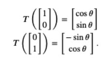
Preserve angles and distances

$$A = \left[\begin{array}{cc}\cos\theta ~~~ -\sin\theta \\\sin\theta ~~~ \cos\theta\end{array} \right]$$

This is easily derived by noting that

ang = np.pi/4
A = np.array([[np.cos(ang), -np.sin(ang)],
              [np.sin(ang),np.cos(ang)]])
print(A)
Xd, Yd = linear_map(A, Xs, Ys)
fig, axs = plt.subplots(1,2)
fig.suptitle('Rotation')
plot_grid(Xs,Ys,axs[0])
plot_grid(Xd,Yd,axs[1])

[[ 0.70710678 -0.70710678]
 [ 0.70710678  0.70710678]]

Similarity (Euclidean): scale, reflection (flip), Rotation and Translations

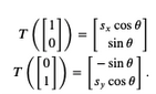
Preserve angles and RATIO between distances

$$A = \left[\begin{array}{cc}s_x\cos\theta ~~~ -\sin\theta \\\sin\theta ~~~ s_y\cos\theta\end{array} \right]$$

This is easily derived by noting that

ang, scale, clip = np.pi/4, 2, True
A = np.array([[scale*np.cos(ang), -np.sin(ang)],
              [np.sin(ang), scale*np.cos(ang)]])
print(A)
Xd, Yd = linear_map(A, Xs, Ys)
fig, axs = plt.subplots(1, 2)
fig.suptitle('Rotation')
plot_grid(Xs, Ys, axs[0])
plot_grid(Xd, Yd, axs[1])
if clip:
    plt.xlim(-nX, nX)
    plt.ylim(-nY, nY)

[[ 1.41421356 -0.70710678]
 [ 0.70710678  1.41421356]]

Affine: shear, scale, reflection (flip), Rotation and Translations

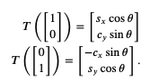
Preserve parallelism (but NOT angles!)

$$A = \left[\begin{array}{cc}s_x\cos\theta ~~~ -c_x\sin\theta \\c_y\sin\theta ~~~ s_y\cos\theta\end{array} \right]$$

This is easily derived by noting that

ang, scale, cx_shear, cy_shear,clip = np.pi/4, 2, 8, 2, False
A = np.array([[scale*np.cos(ang), -cx_shear*np.sin(ang)],
              [cy_shear*np.sin(ang), scale*np.cos(ang)]])
print(A)
Xd, Yd = linear_map(A, Xs, Ys)
fig, axs = plt.subplots(1, 2)
fig.suptitle('Rotation')
plot_grid(Xs, Ys, axs[0])
plot_grid(Xd, Yd, axs[1])
if clip:
    plt.xlim(-nX, nX)
    plt.ylim(-nY, nY)

[[ 1.41421356 -5.65685425]
 [ 1.41421356  1.41421356]]

Hyperplanes

Hyperplane: a generalization to higher dimensions of a line ($D=2$) or of a plane ($D=3$). In a $d$-dimensional vector space, a hyperplane has $d-1$ dimensions and divides the space into two half-spaces.

$$ \mathbf{w}\mathbf{x} + \mathbf{b} = 0 $$

where $\mathbf{w}$ is a vector normal to the hyperplane and $\mathbf{b}$ is an offset

Hyperplanes

Hyperplane: a generalization to higher dimensions of a line ($D=2$) or of a plane ($D=3$). In an $d$-dimensional vector space, a hyperplane has $d-1$ dimensions and divides the space into two half-spaces.

$$ \mathbf{w}\mathbf{x} + \mathbf{b} = 0$$

where $\mathbf{w}$ is a vector normal to the hyperplane and $\mathbf{b}$ is an offset

Projection

Suppose that we have two vectors $\mathbf{v}$ and a column vector $\mathbf{w}=[2,1]^\top$.

We want to project $\mathbf{v}$ onto $\mathbf{w}$ or better project v onto the subspace (line in this case) of $\mathbf{w}$.

Recalling trigonometry, we see the formula $\|\mathbf{v}\|\cos(\theta)$ is the length of the projection of the vector $\mathbf{v}$ onto the direction of $\mathbf{w}$

Projection vector onto subspace defined by $\mathbf{w}$

$$\mathbb{P}_\mathbf{w}(\mathbf{v}) = \frac{\mathbf{w}\mathbf{w}^T}{\mathbf{w}^T\mathbf{w}}\mathbf{v} = \left( \frac{\mathbf{w}}{||\mathbf{w}||}\right)\left(\frac{\mathbf{w}}{||\mathbf{w}||}\right)^T\mathbf{v}$$

Defining a unit vector $\mathbf{\hat{w}}=\frac{\mathbf{w}}{||\mathbf{w}||}$ we have: $$\mathbb{P}_\mathbf{w}(\mathbf{v}) = \underbrace{\mathbf{\hat{w}}}_{\text{direction}} \left(\underbrace{\mathbf{\hat{w}}^T \mathbf{v}}_{\text{length}}\right)$$

• Projection must be on unit vector $\alpha\cdot\mathbf{\hat{w}}$
• How long in this direction? $\alpha=\mathbf{\hat{w}}^T \mathbf{v}$ that gives the length of v onto w.
• $\mathbf{w}$ can be also a matrix, not a vector (a matrix in which columns are vectors).

This lecture material is taken from

• Geometry of the Transformations
• Geometry of Transformations take 2
• This pdf covers this part
• Illustrations and some math parts are taken from d2l.ai, eigendecomposition
• Code for Eigendecomposition

Today's lecture

Decomposition (Eigen, SVD), PCA (we use projection!)

Applications of PCA

Recap on Calculus

⚠️ All the examples are in 2D but generalizes to 3D and N-D

• Machine Learning is about thinking in N-dimensional space
• ...especially for vision problems (images, videos)
• 2D is used for the sake of visualization and clarity in the explanation

Eigendecomposition

Suppose that we have a matrix $A$ with the following entries:

$$ \mathbf{A} = \begin{bmatrix} 2 & 0 \\ 0 & -1 \end{bmatrix}. $$

If we apply $A$ to any vector $\mathbf{v} = [x, y]^\top$, we obtain a vector $\mathbf{A}\mathbf{v} = [2x, -y]^\top$. This has an intuitive interpretation: stretch the vector to be twice as wide in the $x$-direction, and then flip it in the $y$-direction.

However, there are some vectors for which something remains unchanged.

Namely $[1, 0]^\top$ gets sent to $[2, 0]^\top$ and $[0, 1]^\top$ gets sent to $[0, -1]^\top$.

These vectors are still in the same line, and the only modification is that the matrix stretches them by a factor of $2$ and $-1$ respectively. We call such vectors eigenvectors and the factor they are stretched by eigenvalues.

In general, if we can find a number $\lambda$ and a vector $\mathbf{v}$ such that

$$ \underbrace{\mathbf{A}}_{\text{known}}\mathbf{v} = \underbrace{\lambda\mathbf{v}}_{\text{unknown}} $$

We say that $\mathbf{v}$ is an eigenvector for $A$ and $\lambda$ is an eigenvalue.

Finding Eigenvalues

$$(\mathbf{A} - \lambda \mathbf{I})\mathbf{v} = 0.$$

For the equation to happen, we see that $(\mathbf{A} - \lambda \mathbf{I})$ must compress some direction down to zero, hence it is not invertible, and thus the determinant is zero. Thus, we can find the eigenvalues by finding for what $\lambda$ is $\det(\mathbf{A}-\lambda \mathbf{I}) = 0$. Once we find the eigenvalues, we can solve $\mathbf{A}\mathbf{v} = \lambda \mathbf{v}$ to find the associated eigenvector(s).

An Example

Let's see this with a more challenging matrix

$$ \mathbf{A} = \begin{bmatrix} 2 & 1\\ 2 & 3 \end{bmatrix}. $$

If we consider $\det(\mathbf{A}-\lambda \mathbf{I}) = 0$, we see this is equivalent to the polynomial equation $0 = (2-\lambda)(3-\lambda)-2 = (4-\lambda)(1-\lambda)$. Thus, two eigenvalues are $4$ and $1$. To find the associated vectors, we then need to solve

$$ \begin{bmatrix} 2 & 1\\ 2 & 3 \end{bmatrix}\begin{bmatrix}x \\ y\end{bmatrix} = \begin{bmatrix}1x \\ 1y\end{bmatrix} \; \text{and} \; \begin{bmatrix} 2 & 1\\ 2 & 3 \end{bmatrix}\begin{bmatrix}x \\ y\end{bmatrix} = \begin{bmatrix}4x \\ 4y\end{bmatrix} . $$

We can solve this with the vectors $[1, -1]^\top$ and $[1, 2]^\top$ respectively.

eigs, eigvects = np.linalg.eig(
                 np.array([[2, 1],
                           [2, 3]]))
print(f'Eigen val:\n {eigs}', end='\n\n')
print(f'EigenVect vect:\n {eigvects}')
# Note that `numpy` normalizes the eigenvectors to be of length one,
# whereas we took ours to be of arbitrary length.
# Additionally, the choice of the sign is arbitrary.
# However, the vectors computed are parallel 
# to the ones we found by hand with the same eigenvalues.
#help(np.linalg.eig)

Eigen val:
 [1. 4.]

EigenVect vect:
 [[-0.70710678 -0.4472136 ]
 [ 0.70710678 -0.89442719]]

Geometric Interpretation of Eigenvectors

Parametric Unit Sphere

\begin{equation} \Big\{ t \in [0,2\pi]~~|~~ x=\cos(t),y=\sin(t) \Big\} \end{equation}

fig_dim = 10
### Unit Sphere
# Parametric sphere
t = np.linspace(0, 2*np.pi, 100) # seems a circle but it is not (move the resolution to 10)
Xs = np.cos(t)
Ys = np.sin(t)

# Plot
fig, ax = plt.subplots()
fig.set_figheight(fig_dim)
fig.set_figwidth(fig_dim)
plot_points(ax, Xs, Ys, col='blue')
plt.show()

fig_dim = 7
### Unit Sphere
# Parametric sphere
t = np.linspace(0, 2*np.pi, 100) # seems a circle but it is not (move the resolution to 10)
Xs = np.cos(t)
Ys = np.sin(t)

# Plot
fig, ax = plt.subplots()
fig.set_figheight(fig_dim)
fig.set_figwidth(fig_dim)
plot_points(ax, Xs, Ys, col='blue')
plt.show()

Linear Transform to Unit Sphere

• For each point $\mathbf{p}=(x,y)$ apply the transform $\mathbf{A}\mathbf{p}^T$
• Plot the result

• We can do it without using for loop (we used it in the previous lecture)

  • by stacking all p column-wise into a matrix P
  • then doing A@P

• For now, assume:

  • A is square

# Define a transform
limit = 2.5
# Define a transformation
# A = np.array([[1.5, 1], 
#               [1, 1.5]])
A = np.array([[1, -1], 
              [-1, 2]])
print(f'Transformation is\n {A}')

Transformation is
 [[ 1 -1]
 [-1  2]]

# Map points on the surface
Xd, Yd = linear_map(A, Xs, Ys)
# let's map the basis
Xu_d, Yu_d = linear_map(A, np.array([1,0]), np.array([0,1]))
units_d = np.stack((Xu_d, Yu_d),axis=1)
# Compute the eigenvalues and eigenvectors
eigVals, eigVecs = np.linalg.eig(A)
print('eigVals', eigVals, 'eigVecs', eigVecs, sep='\n'*2)

eigVals

[0.38196601 2.61803399]

eigVecs

[[-0.85065081  0.52573111]
 [-0.52573111 -0.85065081]]

# Plot src points and destination points
fig, ax = plt.subplots(1,1)
fig.set_figheight(fig_dim)
fig.set_figwidth(fig_dim)
# Plot src
plot_points(ax, Xs, Ys, col='blue')
# Plot destination
plot_points(ax, Xd, Yd, col='green')
ax.set_aspect('equal')
ax.set_xlim(-limit,limit)
ax.set_ylim(-limit,limit)
# Plot normalized eigenvectors (unit 1)
plotVectors(ax, [eigVecs[:,0], eigVecs[:,1]],
            cols=['red']*2)
# Plot unnormalized eigenvectors (unit 1)
# we have to multiply back to its own eig val
plotVectors(ax, [eigVals[0]*eigVecs[:,0], eigVals[1]*eigVecs[:,1]],
            cols=['pink']*2)
plotVectors(ax, [Xu_d, Yu_d ],
            cols=['gray']*2)

# Plot src points and destination points
fig, ax = plt.subplots(1,1)
fig.set_figheight(fig_dim)
fig.set_figwidth(fig_dim)
# Plot src
plot_points(ax, Xs, Ys, col='blue')
# Plot destination
plot_points(ax, Xd, Yd, col='green')
ax.set_aspect('equal')
ax.set_xlim(-limit,limit)
ax.set_ylim(-limit,limit)
# Plot normalized eigenvectors (unit 1)
plotVectors(ax, [eigVecs[:,0], eigVecs[:,1]],
            cols=['red']*2)
# Plot unnormalized eigenvectors (unit 1)
# we have to multiply back to its own eig val
plotVectors(ax, [eigVals[0]*eigVecs[:,0], eigVals[1]*eigVecs[:,1]],
            cols=['pink']*2)
plotVectors(ax, [Xu_d, Yu_d ],
            cols=['gray']*2)

Interpretations of the determinant with Eigendecomposition

• Symmetric if $A = A^T$ so we can compute eigenvalues
• The determinant of a matrix is the product of the eigenvalues
  • So determinant does not capture change in directions (consider only eigenvalues)
  • Just change in the "hyper-volume" (area in 2D).
• The determinant can be considered as the ratio between
  • Volume of destination shape/volume of the source shape
  • Ratio of area between the ellipse and circle is np.prod(eigVals) =

    NameError: name 'np' is not defined

Eigendecomposition of Matrices

$$ \mathbf{W} = \begin{bmatrix} 1 & 1 \\ -1 & 2 \end{bmatrix}, $$

be the matrix where the columns are the eigenvectors of the matrix $\mathbf{A}$. Let

$$ \boldsymbol{\Sigma} = \begin{bmatrix} 1 & 0 \\ 0 & 4 \end{bmatrix}, $$

be the matrix with the associated eigenvalues on the diagonal. Then the definition of eigenvalues and eigenvectors tells us that

$$ \mathbf{A}\mathbf{W} =\mathbf{W} \boldsymbol{\Sigma} . $$

The matrix $W$ is invertible, so we may multiply both sides by $W^{-1}$ on the right, we see that we may write

$$\mathbf{A} = \mathbf{W} \boldsymbol{\Sigma} \mathbf{W}^{-1}.$$

if $\mathbf{W}$ is invertible

Operations on Eigendecompositions

One nice thing about eigendecompositions is that we can write many operations we usually encounter cleanly in terms of the eigendecomposition. As a first example, consider:

$$ \mathbf{A}^n = \overbrace{\mathbf{A}\cdots \mathbf{A}}^{\text{$n$ times}} = \overbrace{(\mathbf{W}\boldsymbol{\Sigma} \mathbf{W}^{-1})\cdots(\mathbf{W}\boldsymbol{\Sigma} \mathbf{W}^{-1})}^{\text{$n$ times}} = \mathbf{W}\overbrace{\boldsymbol{\Sigma}\cdots\boldsymbol{\Sigma}}^{\text{$n$ times}}\mathbf{W}^{-1} = \mathbf{W}\boldsymbol{\Sigma}^n \mathbf{W}^{-1}. $$

This tells us that for any positive power of a matrix, the eigendecomposition is obtained by just raising the eigenvalues to the same power. The same can be shown for negative powers, so if we want to invert a matrix we need only consider

$$ \mathbf{A}^{-1} = \mathbf{W}\boldsymbol{\Sigma}^{-1} \mathbf{W}^{-1}, $$

or in other words, just invert each eigenvalue.

Spectral Theorem

Informal: Given a matrix $\mathbf{A}$ squared and symmetric, $\mathbf{A} \in \mathbb{R}^{d\times d}$ and $\mathbf{A} = \mathbf{A}^T$ then:

• All the eigenvalues take real values
• The eigenvectors are all orthogonal

Practical applications:

• Hessian, Covariance Matrices
• Kernel matrices, Projection Matrices

Eigendecompositions of Symmetric Matrices

• Hessian
• Covariance Matrices
• PCA
• Kernels etc

Method	$\mathbf{A}$	Decompostion

SVD | any | $\mathbf{A} = \mathbf{U}\mathbf{\Sigma}\mathbf{V}^{\top}$ Eig | square | $\mathbf{A} = \mathbf{U}\mathbf{\Sigma}\mathbf{U}^{-1}$ Eig=SVD | square/sym | $\mathbf{A} = \mathbf{U}\mathbf{\Sigma}\mathbf{U}^{\top}$

Decomposition as a Geometric Pipeline

$$\mathbf{A}\mathbf{x} = \underbrace{(\mathbf{U} \underbrace{(\mathbf{\Sigma}\underbrace{(\mathbf{U}^{-1}\mathbf{x})}_{\text{1st step/rotate}})}_{\text{2nd step/scale}})}_{\text{3rd step/rotate}}$$

Method		Step 1	Step 2	Step 3

geometry | |rotate| scale\reflect| rotate SVD | | $\mathbf{V}^{\top}$ | $\mathbf{\Sigma}$ | $\mathbf{U}$ geometry | |rotate| scale\reflect| rotate Eig | | $\mathbf{U}^{-1}$ | $\mathbf{\Sigma}$ | $\mathbf{U}$

Decomposition as a Geometric Pipeline (Code)

print('A', A, sep='\n\n')
Sigma, U = np.diag(eigVals), eigVecs
print('Sigma', Sigma, 'U', U, sep='\n\n')

A

[[ 1 -1]
 [-1  2]]
Sigma

[[0.38196601 0.        ]
 [0.         2.61803399]]

U

[[-0.85065081  0.52573111]
 [-0.52573111 -0.85065081]]

# Plot src points and destination points
fig, axes = plt.subplots(1, 4)
fig.set_figheight(20)
fig.set_figwidth(20)
# apply [Id, Uinv, Sigma, U]
Trans = [np.diag((1, 1)), U.T, Sigma, U]
titles = ['Init', 'Step 1  Uinv', 'Step 2  Sigma', 'Step 3  U']
X_orig = np.array([1, 0])
Y_orig = np.array([0, 1])
Xss = np.copy(Xs)
Yss = np.copy(Ys)
for count, (ax, T, title) in enumerate(zip(axes, Trans, titles)):
    ax.set_xlim(-limit, limit)
    ax.set_ylim(-limit, limit)
    ax.set_aspect('equal')
    ax.set_title(title)
    Xss, Yss = linear_map(T, Xss, Yss)
    X_orig, Y_orig = linear_map(T, X_orig, Y_orig)
    if count == 0:
        plot_points(ax, Xs, Ys, col='blue')
    unit_v = np.stack((X_orig, Y_orig), axis=1)
    plotVectors(ax, unit_v, ['blue', 'red'])
    plot_points(ax, Xss, Yss, col='green')

# Plot src points and destination points
fig, axes = plt.subplots(1, 4)
fig.set_figheight(20)
fig.set_figwidth(20)
# apply [Id, Uinv, Sigma, U]
Trans = [np.diag((1, 1)), U.T, Sigma, U]
titles = ['Init', 'Step 1  Uinv', 'Step 2  Sigma', 'Step 3  U']
X_orig = np.array([1, 0])
Y_orig = np.array([0, 1])
Xss = np.copy(Xs)
Yss = np.copy(Ys)
for count, (ax, T, title) in enumerate(zip(axes, Trans, titles)):
    ax.set_xlim(-limit, limit)
    ax.set_ylim(-limit, limit)
    ax.set_aspect('equal')
    ax.set_title(title)
    Xss, Yss = linear_map(T, Xss, Yss)
    X_orig, Y_orig = linear_map(T, X_orig, Y_orig)
    if count == 0:
        plot_points(ax, Xs, Ys, col='blue')
    unit_v = np.stack((X_orig, Y_orig), axis=1)
    plotVectors(ax, unit_v, ['blue', 'red'])
    plot_points(ax, Xss, Yss, col='green')

Geometry of SVD

Source: Wikipedia

Principal Component Analysis (PCA)

PCA works in unsupervised learning settings

\begin{equation} \underbrace{\{\mathbf{x}_i\}_{i=1}^N}_{\text{known}} \sim \underbrace{\mathcal{D}}_{\text{unknown}} \end{equation}

Assumptions

• $\mathbf{x}_i \in \mathbb{R}^D$
• $N \geq D$ (number of points higher than number of features; or else, more points than dimensions..for now...)
• $D \geq k$ (where k is the dimension of the subspace on which we will project the points | number of components we will take)

Objective: find a transformation for compressing the data.

What does it mean compressing data? Maybe have different meanings

Which kind of transformation?

########### We know the generative model of the data D ############
np.random.seed(0) # fixing the seed
n_samples=100; cov = [[3, 3], [3, 4]]
# Assumes know the generative model of data
X = np.random.multivariate_normal(mean=[1, 1], cov=cov, size=n_samples)
###########################################################

print(f'num of points {X.shape[0]} in dimension {X.shape[1]}')
fig = plt.figure(figsize=(8,8))
plt.scatter(*X.T) 
plt.scatter(0, 0, c='r', marker='o')
plt.ylabel('Enjoyment')
_ = plt.xlabel('Skills')

num of points 100 in dimension 2

Covariance Matrix: the shape of the input matrix matters

• $\mathbf{X} \in \mathbb{R}^{N\times D}$
• N=samples [rows] in D dimensional space [cols]

NameError: name 'X' is not defined

then the covariance matrix needs to be $ \in \mathbb{R}^{D\times D}$: $$\mbf{C} = \frac{1}{N} (\mathbf{X}-\boldsymbol{\mu})^T(\mathbf{X}-\boldsymbol{\mu}) $$

Covariance Matrix: the shape of the input matrix matters

• $\mathbf{X} \in \mathbb{R}^{D\times N}$
• N=samples [columns] in D dimensional space [row]

NameError: name 'X' is not defined

then the covariance matrix needs to be $ \in \mathbb{R}^{D\times D}$: $$\mbf{C} = \frac{1}{N} (\mathbf{X}-\boldsymbol{\mu})(\mathbf{X}-\boldsymbol{\mu})^T $$

First Step: Standardize the data

• Assumptions that $\mathbf{X}$ is sampled from multi-variate Gaussian distribution
• Center all the data in the center (origin). Compute the mean and remove it.
• [Optional] Rescale all axes so that the standard deviation is one.

$$ \mathbf{X}^{\prime} \leftarrow \frac{\mathbf{X} - \mathbf{\mu}}{\mathbf{\sigma}} $$

After: $ \mathbf{X}^{\prime}$ is standardized

Objective: find a transformation (subspace) for compressing the data

• Which subspace are we going to find? 🤔
• There could be more than one!

Second Step: Finding the components

• PCA finds a subspace that maximizes the variance of the data.
• Given the input $D$-dimensional space, PCA finds a $k$-dimensional subspace that maximizes the variance of data.
• Motivation: compress the dimensions, but keep most of the information i.e. preserve the variance of the data as much as possible

Play a game

I will show you a point cloud,

you tell me STOP when the variance of the data is maximized on the subspace

/>

Taken from StackExchange

• Find $\mathbf{u}\in \mathbb{R}^D $ s.t. $\left\|\mathbf{u}\right\|_2=1$ for which you can project the data $\mathbf{x}^{\prime}=\mathbb{P}_{\mathbf{u}}\mathbf{x}$

$$ \mathbb{P}_{\mathbf{u}}\mathbf{x} = \frac{\mathbf{u}\mathbf{u}^T}{\mathbf{u}^T\mathbf{u}}\mathbf{x} = (\mathbf{x}^T\mathbf{u})\mathbf{u}$$

• We have to maximize the variance once projected.
• Which means making the projection of x with u large:
• We can measure the size of the projection with $\ell_2^2$ norm.

$$\arg\max_{\mathbf{u}} \frac{1}{N}\sum_i^N \left\| \mathbb{P}_{\mathbf{u}}\mathbf{x}_i \right\|_2^2$$

• Find $\mathbf{u}\in \mathbb{R}^k$ s.t. $\left\|\mathbf{u}\right\|_2=1$ for which you can project the data $\mathbf{x}^{\prime}=\mathbb{P}_{\mathbf{u}}\mathbf{x}$

$$ \mathbb{P}_{\mathbf{u}}\mathbf{x} = \frac{\mathbf{u}\mathbf{u}^T}{\mathbf{u}^T\mathbf{u}}\mathbf{x} = (\mathbf{x}^T\mathbf{u})\mathbf{u}$$

• We have to maximize the variance once projected.
• Which means making the projection of x with u large:
• We can measure the size of the projection with $\ell_2$ norm.

$$\arg\max_{\mathbf{u}} \frac{1}{N}\sum_i^N \left\| \mathbb{P}_{\mathbf{u}}\mathbf{x} \right\|_2^2 \rightarrow \arg\max_{\mathbf{u}} \frac{1}{N}\sum_i^N \left\| (\mathbf{x}_i^T\mathbf{u})\mathbf{u}\right\|_2^2$$

$$\arg\max_{\mathbf{u}} \frac{1}{N}\sum_i^N \left\| (\mathbf{x}_i^T\mathbf{u})\mathbf{u}\right\|_2^2=\frac{1}{N}\sum_i^N (\mathbf{x}_i^T\mathbf{u})^2 = \frac{1}{N}\sum_i^N ( \mathbf{x}_i^T\mathbf{u})(\mathbf{x}_i^T\mathbf{u}) = \frac{1}{N}\sum_i^N \underbrace{\mathbf{u}^T\mathbf{x}_i}_{\text{reverse dot prod}}\mathbf{x}_i^T\mathbf{u} = \mathbf{u}^T \left(\frac{1}{N}\sum_i^N \mathbf{x}_i\mathbf{x}_i^T\right)\mathbf{u}$$$$ \arg\max_{\mathbf{u}} \mathbf{u}^T \mathbf{C}\mathbf{u}~~\text{where}~~\mathbf{C}=\frac{1}{N}\mathbf{X}\mathbf{X}^T$$

• So the $\mathbf{u}$ that maximizes the data is the eigenvector of covariance matrix C.
• Remember that $\mathbf{X}$ is "zero mean".
• $\left\|\mathbf{u}\right\|_2=1$

Taken from

StackExchange

Can be used for compressing and reconstructing the data using U up to k components:

$$\underbrace{\mathbf{x}^T}_{\text{rec}} = \underbrace{\underbrace{\mathbf{U}_{|k}}_{k \mapsto D}\quad\underbrace{\underbrace{\mathbf{U}_{|k}^T}_{D \mapsto k}\quad\underbrace{\mathbf{x}^T}_{\text{orig}}}_{projection}}_{reconstruction}$$

Subspaces in decreasing order of variance

$$ (\lambda_1,\mathbf{u}_1),\ldots,(\lambda_d,\mathbf{u}_d) = \text{eig}(\frac{1}{N}\mathbf{X}^T\mathbf{X}) $$

Note: *numpy is not guaranteed to return it ordered so you have to sort*

How do we choose the subspace where to cut the dimension?

• From $D$-dimensional to $k$-dimension
• Given the spectrum $$\mathbf{\Sigma} = \text{diag}(\lambda_1,...,\lambda_d)$$ we can remove the dimension considering the spectrum "energy" and retain e.g. 95% of the variance in data.

That is, keep $k$ components until:

$$\frac{\sum_i^k \lambda_i}{\sum_i^d \lambda_i} \leq 95\%$$

PCA Applications

• Visualization
• Dimensionality Reduction
• Reconstructing data and Compression
• Further pre-processing by machine learning algorithms
• Decorrelate the features

Let's go back to our problem

print(f'num of points {X.shape[0]} in dimension {X.shape[1]}')
fig = plt.figure(figsize=(8,8))
plt.scatter(*X.T, alpha=0.3)
plt.scatter(0, 0, c='red')
plt.ylabel('Enjoyment')
plt.xlabel('Skills')
plt.axis('scaled')
plt.xlim(-6, 6)
plt.ylim(-6, 6)

num of points 100 in dimension 2

(-6.0, 6.0)

# standardize
center = X.mean(axis=0) #X shape is 100x2
std = X.std(axis=0)
Xp = (X-center)/std

fig = plt.scatter(*X.T, alpha=0.3)
plt.scatter(0, 0, c='red')
plt.quiver(0, 0, *center, angles='xy', scale_units='xy', scale=1)
plt.ylabel('Enjoyment')
plt.xlabel('Skills')
plt.axis('scaled')
plt.xlim(-3, 3)
_=plt.ylim(-3, 3)
#print(center)  

fig = plt.figure(figsize=(8,8))
plt.scatter(*Xp.T, alpha=0.3)
plt.scatter(0, 0, c = 'red')
plt.ylabel('Enjoyment')
plt.xlabel('Skills')
plt.axis('scaled')
plt.xlim(-6, 6)
_=plt.ylim(-6, 6)

C = np.cov(X, rowvar=False)
Sigma, U = np.linalg.eig(C)
# If rowvar is True (default), then each row represents a variable, 
# with observations in the columns. Otherwise, the relationship 
# is transposed: each column represents a variable, while the 
# rows contain observations.

C.shape

(2, 2)

Sigma.shape, U.shape, Sigma

((2,), (2, 2), array([0.47772418, 6.90110921]))

total_energy = Sigma.sum()
var_exp = Sigma/total_energy
cum_var_exp = np.cumsum(var_exp)

plt.bar(range(len(var_exp)), var_exp, alpha=0.5, align='center',
        label='individual explained variance')
plt.step(range(len(var_exp)), cum_var_exp, where='mid',
         label='cumulative explained variance')
plt.ylabel('Explained variance ratio')
plt.xlabel('Principal components')
plt.legend(loc='best')
plt.tight_layout()
plt.show()
Sigma = np.diag(Sigma)

PCA for projecting/reconstructing data

No compression, no rotation

Can be seen as reconstructing the data using U: $$\underbrace{\mathbf{x}^T}_{2 \times N} = \underbrace{\mathbf{U}}_{2\times 2}\quad\underbrace{\mathbf{U}^T}_{2\times 2}\quad\underbrace{\mathbf{x}^T}_{2\times N}$$

# Full projection
print(U.shape, U.T.shape, Xp.T.shape)
Xd = U @ U.T @ Xp.T  # Our transformation
print(Xd.shape)

(2, 2) (2, 2) (2, 100)
(2, 100)

print('Sigma', Sigma, 'U', U, sep='\n\n')

Sigma

[[0.47772418 0.        ]
 [0.         6.90110921]]

U

[[-0.76738982 -0.64118083]
 [ 0.64118083 -0.76738982]]

What happens if we use only the first dominant basis (first component)?

Utrunc = U[:,1].reshape(2,-1) # need reshape for matrix mul.
# note [:,1] selects the eigenvector with more energy (highest eigen value)
# if you have more of them you have to sort, with 2 it is easier it is either this or the other
print()

# Compressed projection
print('Full projection>', U.shape, U.T.shape, Xp.T.shape)
print('Compressed projection>', Utrunc.shape, Utrunc.T.shape, Xp.T.shape)
Xd = Utrunc.T @ Xp.T  # Our transformation project down = Utrunc.T @ x.T;
print(Xd.shape)

Full projection> (2, 2) (2, 2) (2, 100)
Compressed projection> (2, 1) (1, 2) (2, 100)
(1, 100)

fig = plt.figure(figsize=(8,1))
plt.plot(Xd[0, ...].T, [0]*Xd.shape[1], 'o')
_ = plt.ylim(-0.001, 0.001)

fig = plt.figure(figsize=(8,8))
plt.scatter(*Xp.T, alpha=0.3)
plt.scatter(0, 0, c = 'red')
plt.ylabel('Enjoyment')
plt.xlabel('Skills')
plt.axis('scaled')
plt.xlim(-6, 6)
_=plt.ylim(-6, 6)

# Compressed projection and back-projected
print(U.shape, U.T.shape, Xp.T.shape)
Xd = Utrunc @ Utrunc.T @ Xp.T  # Our transformation A = U @ Ut;
print(Xd.shape)

(2, 2) (2, 2) (2, 100)
(2, 100)

fig, ax = plt.subplots()
fig.set_figheight(8)
fig.set_figwidth(8)
ax.scatter(*Xp.T, alpha=0.3)
ax.scatter(*Xd, color='green', alpha=0.5)
_ = ax.quiver(*Xp.T, *(Xd-Xp.T), alpha=0.2, linestyle='dashed',
          linewidth=.4, color='black')  # start, end-start

We have reduced the dimensionality of the data since we projected on a line

Can be used for compressing and reconstructing the data using U up to k components: $$\underbrace{\mathbf{x}^T}_{\text{rec}} = \underbrace{\underbrace{\mathbf{U}_{|k}}_{k \mapsto D}\quad\underbrace{\underbrace{\mathbf{U}_{|k}^T}_{D \mapsto k}\quad\underbrace{\mathbf{x}^T}_{\text{orig}}}_{projection}}_{reconstruction}$$

PCA Full recipe

$$ \mathbf{X}^{\prime} \leftarrow \frac{\mathbf{X} - \mathbf{\mu}}{\boldsymbol{\sigma}} $$$$\underbrace{\mathbf{x}^{T\prime}_p}_{\text{rec}} = \underbrace{\underbrace{\mathbf{U}_{|k}}_{k \mapsto D}\quad\underbrace{\underbrace{\mathbf{U}_{|k}^T}_{D \mapsto k}\quad\underbrace{\mathbf{x}^{T\prime}}_{\text{orig}}}_{projection}}_{reconstruction}$$$$ \mathbf{x}_p\leftarrow\left(\mathbf{x}^{T\prime}_p{\boldsymbol{\sigma}}\right)+\mathbf{\mu}$$

Example: DNA Analysis

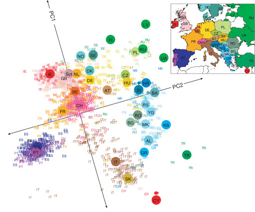
Even linear dimensionality reduction is powerful. Here, in uncovers the geography of European countries from only DNA data

Machine Learning

---

3. PCA in higher dimension, 3DMM, the curse of dimensionality

Iacopo Masi

Recap previous lectures

• Vector and Matrix as a formal way to represent data
• Why LA? (data, covariance matrix, calculus)
• Operations (vector to vector, matrix to vector, inner product)
• Geometric Interpretation of the inner product
• Subspaces/Rank/Inverse
• Projection onto a subspace

This lecture material is taken from

• ### Note: you can find PCA on Chapter 12 of [Bishop Book]
• Geometry of the Transformations
• Geometry of Transformations take 2
• This pdf covers this part
• Illustrations and some math parts are taken from d2l.ai, eigendecomposition
• Code for Eigendecomposition

Today's lecture

Recall PCA (we use projection!) and Eigendecomposition

Note: you can find PCA on Chapter 12 of [Bishop Book]

Applications of PCA (3DMM)

PCA Full recipe

$$ \mathbf{X}^{\prime} \leftarrow \frac{\mathbf{X} - \mathbf{\mu}}{\boldsymbol{\sigma}} $$$$\underbrace{\mathbf{x}^{T\prime}_p}_{\text{rec}} = \underbrace{\underbrace{\mathbf{U}_{|k}}_{k \mapsto D}\quad\underbrace{\underbrace{\mathbf{U}_{|k}^T}_{D \mapsto k}\quad\underbrace{\mathbf{x}^{T\prime}}_{\text{orig}}}_{projection}}_{reconstruction}$$$$ \mathbf{x}_p\leftarrow\left(\mathbf{x}^{T\prime}_p{\boldsymbol{\sigma}}\right)+\mathbf{\mu}$$

########################################
plt.figure(figsize=(8,8))
plt.scatter(*X.T, alpha=0.3)
plt.scatter(0, 0, c='red')
plt.ylabel('Enjoyment')
plt.xlabel('Skills')
plt.axis('scaled')
plt.xlim(-6, 6)
plt.ylim(-6, 6)
# Taking reconstructed data and shift it back
###############################
Xd_back = (Xd.T*std)+center
#########################
plt.scatter(*Xd_back.T, color='green', marker='.')

<matplotlib.collections.PathCollection at 0x7fd3e18fe760>

Application: PCA to rotate data (make it axis aligned), decorrelate data

in unsupervised way

• For reading images there are multiple library
• One is Pillow conda install pillow or pip install pillow

from PIL import Image
import requests
from io import BytesIO

#response = requests.get('https://cdn-icons-png.flaticon.com/512/24/24335.png')
img = Image.open('figs/italy.png')
im = np.array(img)

img

X, Y = np.where(im != 0)
sampling = 100  # to have less points
X, Y = X[::sampling], Y[::sampling]

fig = plt.scatter(X, Y, c=X, marker='o', cmap='jet')
plt.scatter(0, 0, c='red')
_ = plt.axis('scaled')

PCA Application - Rotate the data and decorrelate them - No compression

$$ \mathbf{X}^{\prime} \leftarrow \frac{\mathbf{X} - \mathbf{\mu}}{\mathbf{\sigma}} $$$$\underbrace{\mathbf{x}^{T\prime}_p}_{\text{rot}} = {\mathbf{U}^T}\quad\underbrace{\mathbf{x}^{T\prime}}_{\text{orig}}$$$$ \text{Optional:}~~~~ \mathbf{x}_p\leftarrow\left(\mathbf{x}^{T\prime}_p{\mathbf{\sigma}}\right)+\mathbf{\mu}$$

pts = np.stack((X, Y), axis=1)
# Nx2
print(f'num of points {pts.shape[0]} in dimension {pts.shape[1]}' )

num of points 746 in dimension 2

# Standardize the data 
# (x-mu)/sigma
center = pts.mean(axis=0)
std = pts.std(axis=0)
pts_z = (pts - center)/std

fig = plt.scatter(*pts_z.T, c=X, marker='.', cmap='jet')
plt.scatter(0,0,c='red')
_ = plt.axis('scaled')

# np.cov wants features on rows
cov = np.cov(pts_z, rowvar=False)
Sigma, U = np.linalg.eig(cov)

# plot principal components aka eigenvectors
fig = plt.scatter(*pts_z.T, c=X, marker='.', cmap='jet')
plt.scatter(0,0,c='red')
plotVectors(fig.axes, [Sigma[0]*U[:,0], Sigma[1]*U[:,1]], cols=['green','blue'])
_ = plt.axis('scaled')

# rotate points
rot = U.T@pts_z.T
np.cov(rot,rowvar=True)

array([[ 3.95280931e-01, -2.38437160e-18],
       [-2.38437160e-18,  1.60740363e+00]])

fig, ax = plt.subplots(1,2)
fig.set_figheight(12)
fig.set_figwidth(12)
# First
ax[0].scatter(*pts_z.T, c=X, marker='.', cmap='jet')
ax[0].scatter(0,0,c='red')
plotVectors(ax[0], [Sigma[0]*U[:,0], Sigma[1]*U[:,1]], cols=['green','blue'])
ax[0].set_aspect('equal')
ax[0].set_xlim(-3,3)
ax[0].set_ylim(-3,3)
# second
ax[1].scatter(*rot, c=X, marker='.', cmap='jet')
ax[1].scatter(0,0,c='red')
plotVectors(ax[1], [Sigma[0]*np.array([1,0]), Sigma[1]*np.array([0,1])], cols=['green','blue'])
ax[1].set_aspect('equal')
ax[1].set_xlim(-3,3)
ax[1].set_ylim(-3,3)

(-3.0, 3.0)

np.set_printoptions(suppress=True) #suppress scientific notation, please watch out using this
np.cov(rot, rowvar=True) # rowvar is True because matrix is 2xN
# do you know why we get this? and what are the values inside?

array([[ 0.39528093, -0.        ],
       [-0.        ,  1.60740363]])

Application: Data whitening

What does it mean whitening or sphering?

Do you remember this?

Graphics from Wikipedia

PCA Application - Whitening - No compression

$$ \mathbf{X}^{\prime} \leftarrow \frac{\mathbf{X} - \mathbf{\mu}}{\mathbf{\sigma}} $$$$\underbrace{\mathbf{x}^{T\prime}_p}_{\text{dec.}} = {\mathbf{\Sigma}^{-1/2}\mathbf{U}^T}\quad\underbrace{\mathbf{x}^{T\prime}}_{\text{orig}}$$

Sigma_inv_sqrt = np.diag(Sigma**-0.5)
# data is rotated and decorrelated (whitening or sphering)
rot_withening = Sigma_inv_sqrt @ U.T @ pts_z.T

fig, ax = plt.subplots(1,3)
fig.set_figheight(14)
fig.set_figwidth(14)
# First
ax[0].scatter(*pts_z.T, c=X, marker='.', cmap='jet')
ax[0].scatter(0,0,c='red')
plotVectors(ax[0], [Sigma[0]*U[:,0], Sigma[1]*U[:,1]], cols=['green','blue'])
ax[0].set_aspect('equal')
ax[0].set_xlim(-3,3)
ax[0].set_ylim(-3,3)
# second
ax[1].scatter(*rot, c=X, marker='.', cmap='jet')
ax[1].scatter(0,0,c='red')
plotVectors(ax[1], [Sigma[0]*np.array([1,0]), Sigma[1]*np.array([0,1])], cols=['green','blue'])
ax[1].set_aspect('equal')
ax[1].set_xlim(-3,3)
ax[1].set_ylim(-3,3)
# third
ax[2].scatter(*rot_withening, c=X, marker='.', cmap='jet')
ax[2].scatter(0,0,c='red')
plotVectors(ax[2], [np.array([1,0]), 
                    np.array([0,1])], cols=['green','blue'])
ax[2].set_aspect('equal')
ax[2].set_xlim(-3,3)
ax[2].set_ylim(-3,3)

(-3.0, 3.0)

fig, ax = plt.subplots(1,3); sizeim=40;
fig.set_figheight(sizeim)
fig.set_figwidth(sizeim)
# First
ax[0].scatter(*pts_z.T, c=X, marker='o', cmap='jet')
ax[0].scatter(0,0,c='red')
plotVectors(ax[0], [Sigma[0]*U[:,0], Sigma[1]*U[:,1]], cols=['green','blue'])
ax[0].set_aspect('equal')
ax[0].set_xlim(-3,3)
ax[0].set_ylim(-3,3)
# second
ax[1].scatter(*rot, c=X, marker='o', cmap='jet')
ax[1].scatter(0,0,c='red')
plotVectors(ax[1], [Sigma[0]*np.array([1,0]), Sigma[1]*np.array([0,1])], cols=['green','blue'])
ax[1].set_aspect('equal')
ax[1].set_xlim(-3,3)
ax[1].set_ylim(-3,3)
# third
ax[2].scatter(*rot_withening, c=X, marker='o', cmap='jet')
ax[2].scatter(0,0,c='red')
plotVectors(ax[2], [np.array([1,0]), 
                    np.array([0,1])], cols=['green','blue'])
ax[2].set_aspect('equal')
ax[2].set_xlim(-3,3)
ax[2].set_ylim(-3,3)

(-3.0, 3.0)

Sanity Check

We take the decorrelated data points and compute the covariance matrix:

$$\mathbf{X}_p\mathbf{X}_p^T$$

if decorrelated should get us:

$$ \begin{bmatrix} 1 & 0 \\ 0 & 1 \end{bmatrix} $$

and in more dimensions should give us $\mathbf{I}$ matrix (identity matrix)

np.cov(rot_withening, rowvar=True) # rowvar is True becausse matrix is 2xN

array([[ 1., -0.],
       [-0.,  1.]])

We can also "prove" it that induced decorrelated and "sphered" points:

$$\underbrace{\mathbf{x}^{T\prime}_p}_{\text{dec.}} = {\mathbf{\Sigma}^{-1/2}\mathbf{U}^T}\quad\underbrace{\mathbf{x}^{T\prime}}_{\text{orig}}$$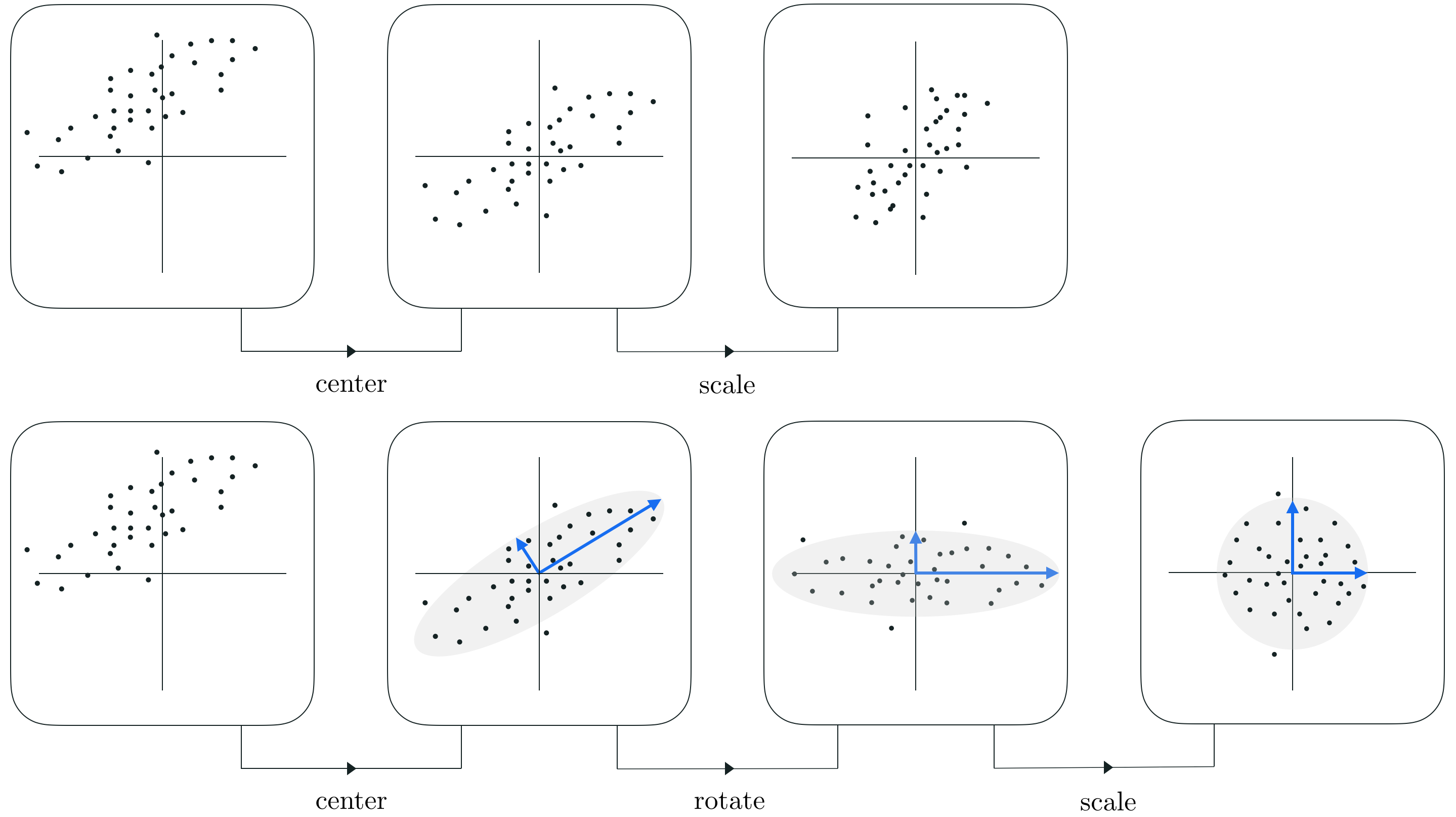

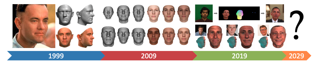
Sphering vs Standardization

PCA in Computer Graphics: 3D Morphable Models (3DMM)

• A set of 3D faces point cloud matrix $\mathbf{X}=\{\mathbf{S}_i\}_{i=1}^M$ with $\mathbf{S}_i \in \mathbf{R}^{3N}$ and $M$ are the samples we have.
• $\mathbf{S}_i = [x_1,y_1,z_1,\ldots,x_N,y_N,z_N,]$ point cloud stack in a vector.
• Assumption: The point cloud is vertex-aligned (usually this implies dense registration, not easy to achieve)
• Assumption: $\mathbf{S}\sim\mathcal{N}(\mathbf{\mu},\mathbf{\Sigma})$ faces are modeled as a multivariate Gaussian distribution.

Figure Credit 3DMM, Past Present and Future

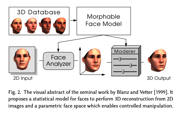
Credits Blanz and Vetter, 1999

3D Face modeling with PCA

$ \mbf{S}^{\prime} = \mbf{\hat{S}} + \sum_{i}^{M-1} \alpha_i \mbf{U}_i $ where:

• $ \mbf{\hat{S}} $ is the mean shape
• and $\mbf{U}_i$ are the $M-1$ principal components that you can compute by learning PCA on $\mbf{X}=\{\mbf{S}_i\}_{i=1}^M$

A (new) 3D face is defined once you know $\mbf{\alpha}$

• $ \mbf{\alpha} = [\alpha_1,\ldots,\alpha_k]$ scales each principal component
• Similar to say:
  • OK, this is the average face (fixed for everyone)
  • but I want to edit the average to add 0.25 * male (1st component) + -0.12 * caucasian (2nd component) + ...

3D Face modeling with PCA

$ \mbf{S}^{\prime} = \mbf{\hat{S}} + \sum_{i}^{M-1} \alpha_i \mbf{U}_i $ where:

PCA assumes the data generation process is a multivariate Gaussian distribution (i.e. a Gaussian/Normal distribution but in 3N-D).

$ \underbrace{\{\mathbf{S}_i\}_{i=1}^M}_{\text{known}} \sim \underbrace{\mathcal{N}(\mbf{\hat{S}},\mbf{Cov}_S)}_{\text{multivariate Gaussian assumption}} \approx \underbrace{\mathcal{D}}_{\text{unknown}} $

• Given a face $\mbf{\alpha} = [\alpha_1,\ldots,\alpha_k]$ you can compute how much it is likely of "being a face" under $\mathcal{N}(\mbf{\hat{S}},\mbf{Cov}_S)$
• $\mbf{\alpha} = [0.2,\ldots,0.24]$ is more probable of being a face (you get something regular)
• $\mbf{\alpha} = [0.1,\ldots,-1.24]$ is less probable of being a face (you get something irregular)

Principal Components refers to Variations in Faces

• 1st component: gender or age (most variation)
• 2nd component: face size (moderate variation)
• .....
• last component: nose size etc (least variation)

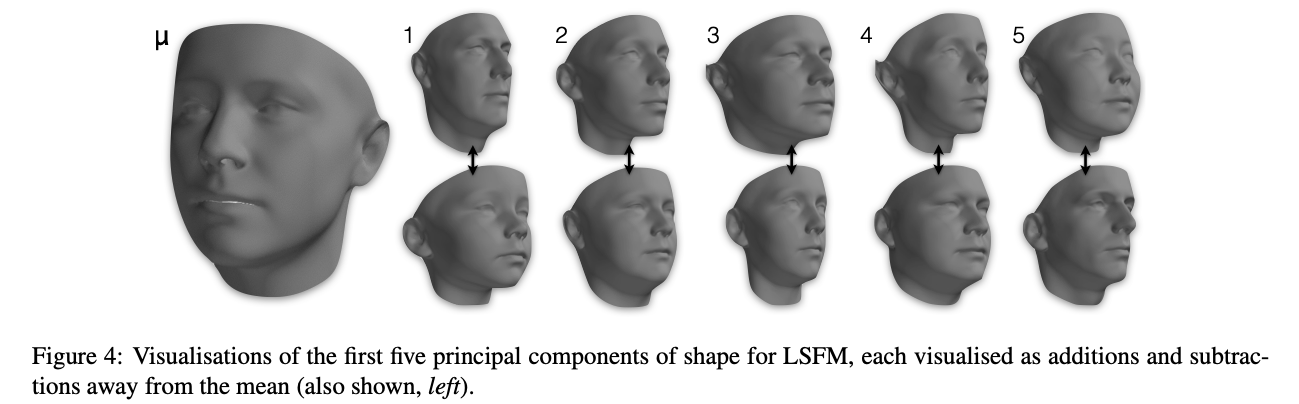
Figure credit Booth et al. 3DMM in the Wild

Click here for interactive demo - FLAME - Max Planck

Expressiveness

$\mbf{S}^{\prime} = \mbf{\hat{S}} + \sum_{i}^{M-1} \alpha_i \mbf{U}_i$ where:

• $ \mbf{\hat{S}} $ is the mean shape
• and $\mbf{U}_i$ are the $ M-1 $ principal components that you can compute by learning PCA on $\mbf{X}=\{\mbf{S}_i\}_{i=1}^M$.

Part-based 3DMM

• The expressiveness of the model can be increased by dividing faces into independent sub-regions that are morphed independently, for example into eyes, nose, mouth and a surrounding region.
• Since all faces are assumed to be in correspondence, it is sufficient to define these regions on a reference face. This segmentation is equivalent to sub-dividing the vector space of faces into independent subspaces.
• A complete 3D face is generated by computing linear combinations for each segment separately and blending them at the borders according to an algorithm proposed for images by a blending algorithm

Two more real world examples

Morphable Models are everywhere - Snapfeet App

Body Morphable Models @ Max Planck Institute for Intelligent Systems

Up next: PCA in High Dimensional Space

• Demonstration with images
• You can think of an image $\mathbf{I}\in \mathbb{R}^{W\times H}$ as a point/vector in high dimension.
• For an image $128\times 128$ now our $D$ dimension is very high. $D=128^2=(2^7)^2=2^{14}\approx16K$

• Let's double the image $128 \mapsto 256$

• For an image $256\times 256$ now our $D$ dimension is very high. $D=256^2=(2^8)^2=2^{16}\approx65K$
• Doubling a side, increases the dimension four times, for two-dimensional nature of images.

PCA is in sklearn but implementing it manually is for understanding

from sklearn.decomposition import PCA
pca = PCA(n_components=2)
pca.fit(X)

In case you have to use it in industry/thesis, you will rely on sklearn

i.e. "not reinventing the wheel" but academically it is good to do it manually