There is not a single textbook but suggested are:
| Topic | Authors | Book |
|---|---|---|
| Generic ML | H. Daumé III | "A Course in Machine Learning", download the book |
| Generic ML | Christopher M. Bishop | “Pattern Recognition and Machine Learning” download the book |
| Generic ML | Kevin P. Murphy | “Probabilistic Machine Learning: An introduction", MIT Press, 2021 |
| Deep Learning | Ian Goodfellow and Yoshua Bengio and Aaron Courville | “Deep Learning”, MIT Press 2016 |
| Deep Learning | Ston Zhang, Zack C. Lipton, Mu Li, Alex J. Smola | “Dive into Deep Learning” |
You can find online most of these or part of them.
NumPy is a library for the Python programming language, adding support for large, multi-dimensional arrays and matrices, along with a large collection of high-level mathematical functions to operate on these arrays
![]()
import numpy as np
x = np.array([[2.5, 3.2], [0, 1], [2, -3]], dtype=np.float32)
print(x)
print(f"Shape {x.shape}")  # the shape is...
print(f"Number of dimensions: {x.ndim}")  # is a matrix (2 axis)
print(f"Number of elements: {x.size}")  # with 6 elements

v = np.array([2.5, 3.2])  # used later
[[ 2.5  3.2]
 [ 0.   1. ]
 [ 2.  -3. ]]
Shape (3, 2)
Number of dimensions: 2
Number of elements: 6
import matplotlib
import matplotlib.pyplot as plt
import numpy as np

v = np.array([2.5, 3.2])
# all the X first, then all the Y
#        [X1   X2]    [Y1  Y2]
plt.plot([0, v[0]], [0, v[1]],
         marker='x', color='red', lw=4,
         markersize=6)
import matplotlib
import matplotlib.pyplot as plt
import numpy as np
%matplotlib inline
plt.style.use('seaborn-v0_8-white')
font = {'family': 'sans-serif',
        'weight': 'bold',
        'size': 22}
matplotlib.rc('font', **font)

# Plotting
plt.figure(figsize=(10, 10))
plt.plot(v[0], v[1], marker='x', color='red', lw=4, markersize=6)
# all the X first, then all the Y
plt.plot([0, v[0]], [0, v[1]], marker='x', color='red', lw=4, markersize=6)
# Eyecandy
plt.axis('equal')
plt.xlabel('x-axis')
plt.ylabel('y-axis')
plt.axhline(0, color='black')
plt.axvline(0, color='black')
plt.title("Vector")
plt.annotate('(0, 0)', xy=(0, 0), xytext=(.1, -.3))
plt.annotate(f'({v[0]},{v[1]})', xy=(v[0], v[1]), xytext=(v[0], v[1]))
plt.axis([-5, 5, -5, 5])
plt.show()

Given a vector, the first interpretation that we should give it is as a point in space.
In two or three dimensions, we can visualize these points by using the components of the vectors to define the location of the points in space compared to a fixed reference called the origin.

This geometric point of view allows us to consider the problem on a more abstract level. No longer faced with some insurmountable seeming problem like classifying pictures as either cats or dogs but separate points in space.
Problem -> Formalization -> Math -> Computational System
Taken from d2l.ai
In parallel, there is a second point of view
that people often take of vectors: as directions in space.
Not only can we think of the vector $\mathbf{v} = [3,2]^\top$
as the location $3$ units to the right and $2$ units up from the origin,
We can also think of it as the direction itself
to take $3$ steps to the right and $2$ steps up.
In this way, we consider all the vectors in the figure the same.

One of the benefits of this shift is that we can make visual sense of the act of vector addition. In particular, we follow the directions given by one vector, and then follow the directions given by the other, as is seen below (rule of the parallelogram).

Difference is just $\mathbf{A}-\mathbf{B}=\mathbf{A}+(-\mathbf{B})$
Taken from [d2l.ai]
$ \mathbf{I}_3 = \begin{bmatrix} 1 & 0 & 0 \\ 0 & 1 & 0 \\ 0 & 0 & 1 \\ \end{bmatrix} $
$\mathbf{I}_3 = \text{diag}(1) $
#help(np.diag)
A = np.ones((3)) #firstly create a vector [1,1,1] and then makes it a diagonal matrix
print(A)
[1. 1. 1.]
Trace is the sum of the diagonal elements
$$ \text{trace}(\mathbf{A}) = \sum_i A_{ii}$$# is ID symmetric?
ID = np.diag(np.ones(3))
np.a ll(ID == ID.T) # == does the comparison element-wise
True
# Generate array from 0 to 8 of int64
# reshape it in a 3x3 matrix
A = np.arange(9).reshape(3, 3)
print(f'A is \n {A}', end='\n'*2)
print(f'The transpose of A is \n {A.T}', end='\n'*2)
print(f'A is if type {A.dtype}')
A is
 [[0 1 2]
 [3 4 5]
 [6 7 8]]

The transpose of A is
 [[0 3 6]
 [1 4 7]
 [2 5 8]]

A is if type int64
Sum all the values across rows (rows will disappear) Sum all values across axis 0.
[ a11 a12 a13
  a21 a22 a23 ]
⬇️ ⬇️ ⬇️
⬇️ ⬇️ ⬇️$R=2, C=3$
$\mathbf{s}_c = \sum_{r=1}^R \mathbf{A}_{rc}, \forall c \in C $
$\mathbf{s}$ is $1 \times C = 1 \times 3= 3.$
print(A,end='\n\n')
# Possible to do a reduction on the matrix (sum along rows)
A_c = A.sum(axis=0, keepdims=False)  # 3 (rows are canceled out)
A_c.shape
print(A_c)
[[0 1 2]
 [3 4 5]
 [6 7 8]]

[ 9 12 15]
# Works for other operations too like mean (average)
A.mean(axis=0, keepdims=False)  # 3 (rows are canceled out)
array([3., 4., 5.])
A = np.arange(9).reshape(3, 3)
B = np.ones_like(A)
C = A + B # if now you have all 1 you can also get the same with A + 1 and will do
print('C', C, 'A', A, 'B', B, sep='\n\n')
np.allclose(C, A+1) # you can sum matrix + scalar, numpy will broadcast
C

[[1 2 3]
 [4 5 6]
 [7 8 9]]

A

[[0 1 2]
 [3 4 5]
 [6 7 8]]

B

[[1 1 1]
 [1 1 1]
 [1 1 1]]
True
A = np.arange(9).reshape(3,3)
B = np.zeros_like(A) #np.ones_like(A)*1.5
C = A * B # Hadamard product (multply element-wise)
print('C',C,'A',A,'B',B,sep='\n\n')
np.allclose(C, A*0)
C

[[0 0 0]
 [0 0 0]
 [0 0 0]]

A

[[0 1 2]
 [3 4 5]
 [6 7 8]]

B

[[0 0 0]
 [0 0 0]
 [0 0 0]]
True
Sum all the values across cols (cols will disappear) Sum all values across axis 1.
a11 a12 a13
a21 a22 a23
➡️ ➡️ ➡️
➡️ ➡️ ➡️$R=2, C=3$
$\mathbf{s}_r = \sum_{c=1}^C \mathbf{A}_{rc}, \forall r \in R $
$\mathbf{s}$ is $R \times 1 = 2 \times 1= 2$
# Sum all the values across cols (cols will disappear)
# Sum all values across axis 1.
print(A)
A.sum(axis=(0,1), keepdims=False) #3 (cols are cancelled out)
[[0 1 2]
 [3 4 5]
 [6 7 8]]
36
a11 a12 a13
a21 a22 a23$ \mathbf{s}_c= \sum_{r=1}^R \mathbf{A}_{rc}, \forall c \in C $
$\mathbf{s}$ is $1 \times C = 1 \times 3$
# Works for other operations too like mean (average)
A.mean(axis=0, keepdims=True) #1x3 (rows are cancelled out but row axis is NOT dropped)
array([[3., 4., 5.]])
x1 x2 x3 x4
           y1
           y2   =    result (dot_product)
           y3
           y4


dot_product = x1y1 + x2y2 + x3y3 + x4y4x = np.array([1, 2, 3])
y = np.array([1, 0, 1])
np.dot(x, y) == np.sum(x*y)
True
The dot product also admits a geometric interpretation: it is closely related to the angle between two vectors.

With some simple algebraic manipulation, we can rearrange terms to obtain
$$ \theta = \arccos\left(\frac{\mathbf{v}^T\cdot\mathbf{w}}{\|\mathbf{v}\|\|\mathbf{w}\|}\right). $$This is a nice result since nothing in the computation references two-dimensions.
Indeed, we can use this in three or three million dimensions without issue.
def angle(v, w):
    return np.arccos(v.dot(w) / (np.linalg.norm(v) * np.linalg.norm(w)))

angle(np.array([0, 1, 2]), np.array([2, 3, 4])) # the result is in radians
0.4189900840328574
In ML contexts where the angle is employed to measure the closeness of two vectors, practitioners adopt the term cosine similarity to refer to the portion $$ \cos(\theta) = \underbrace{\frac{\mathbf{v}^T\cdot\mathbf{w}}{\|\mathbf{v}\|\|\mathbf{w}\|}}_{\text{cosine similarity}}. $$
           P           ____________________
      y1 y2 y3 y4     | x1 * yi for each Y |
   x1                 |                    |
D  x2              =  |                    |
x3 |___________________ |x = np.array([1, 2, 3])
y = np.array([1, 0, 1, -1])
np.outer(x,y)
array([[ 1,  0,  1, -1],
       [ 2,  0,  2, -2],
       [ 3,  0,  3, -3]])
$\mathbf{A} \in \mathbb{R}^{m \times n} ~~$ $\mathbf{x} \in \mathbb{R}^{n \times 1}$
$\mathbf{A}\mathbf{x} =\mathbf{b}$
$$ \mathbf{A} = \begin{bmatrix} a_{11} & \ldots & a_{1n} \\ \ldots & & \ldots \\ a_{m1}& \ldots& a_{mn} \\ \end{bmatrix}~~ \mathbf{x} = \begin{bmatrix} x_{11} \\ \ldots \\ x_{n1} \\ \end{bmatrix} $$Take each row of A, that is $\mathbf{a}_r^T$, then do inner product with $\mathbf{x}$ $$ \mathbf{b} = \begin{bmatrix} \mathbf{a}_1^T\mathbf{x} \\ \ldots \\ \mathbf{a}_m^T\mathbf{x} \\ \end{bmatrix} $$
Take each value of $\mathbf{x}$, scale each column of A; sum across cols (axis=1).
For example, we can represent rotations as multiplications by a square matrix and rotate points.
A = np.arange(27).reshape(3, 9)
x = np.ones((9, 1))
b = A @ x  # 3x9 @ 9x1 = 3x1
bb = np.matmul(A, x)
bbb = np.dot(A,x)
print('A', A, 'x', x, 'b', b, 'bb', bb,'bbb', bbb, sep='\n\n')

# Questions for you: A*B does elementwise multiplcation # will it work?
A

[[ 0  1  2  3  4  5  6  7  8]
 [ 9 10 11 12 13 14 15 16 17]
 [18 19 20 21 22 23 24 25 26]]

x

[[1.]
 [1.]
 [1.]
 [1.]
 [1.]
 [1.]
 [1.]
 [1.]
 [1.]]

b

[[ 36.]
 [117.]
 [198.]]

bb

[[ 36.]
 [117.]
 [198.]]

bbb

[[ 36.]
 [117.]
 [198.]]
We have two matrices $\mathbf{A} \in \mathbb{R}^{n \times k}$ and $\mathbf{B} \in \mathbb{R}^{k \times m}$:
Let $\mathbf{a}^\top_{i} \in \mathbb{R}^k$ denote the row vector representing the $i^\mathrm{th}$ row of the matrix $\mathbf{A}$ and let $\mathbf{b}_{j} \in \mathbb{R}^k$ denote the column vector from the $j^\mathrm{th}$ column of the matrix $\mathbf{B}$:
$$\mathbf{A}= \begin{bmatrix} \mathbf{a}^\top_{1} \\ \mathbf{a}^\top_{2} \\ \vdots \\ \mathbf{a}^\top_n \\ \end{bmatrix}, \quad \mathbf{B}=\begin{bmatrix} \mathbf{b}_{1} & \mathbf{b}_{2} & \cdots & \mathbf{b}_{m} \\ \end{bmatrix}. $$To form the matrix product $\mathbf{C} \in \mathbb{R}^{n \times m}$, we simply compute each element $c_{ij}$ as the dot product between the $i^{\mathrm{th}}$ row of $\mathbf{A}$ and the $j^{\mathrm{th}}$ row of $\mathbf{B}$, i.e., $\mathbf{a}^\top_i \mathbf{b}_j$:
$$\mathbf{C} = \mathbf{AB} = \begin{bmatrix} \mathbf{a}^\top_{1} \\ \mathbf{a}^\top_{2} \\ \vdots \\ \mathbf{a}^\top_n \\ \end{bmatrix} \begin{bmatrix} \mathbf{b}_{1} & \mathbf{b}_{2} & \cdots & \mathbf{b}_{m} \\ \end{bmatrix} = \begin{bmatrix} \mathbf{a}^\top_{1} \mathbf{b}_1 & \mathbf{a}^\top_{1}\mathbf{b}_2& \cdots & \mathbf{a}^\top_{1} \mathbf{b}_m \\ \mathbf{a}^\top_{2}\mathbf{b}_1 & \mathbf{a}^\top_{2} \mathbf{b}_2 & \cdots & \mathbf{a}^\top_{2} \mathbf{b}_m \\ \vdots & \vdots & \ddots &\vdots\\ \mathbf{a}^\top_{n} \mathbf{b}_1 & \mathbf{a}^\top_{n}\mathbf{b}_2& \cdots& \mathbf{a}^\top_{n} \mathbf{b}_m \end{bmatrix}. $$We can think of the matrix-matrix multiplication $\mathbf{AB}$ as performing $m$ matrix-vector products or $m \times n$ dot products and stitching the results together to form an $n \times m$ matrix.
The term matrix-matrix multiplication is often simplified to matrix multiplication, and should not be confused with the Hadamard product (element-wise product).
Taken from d2l.ai
A = np.random.rand(3, 5)
B = np.random.rand(5, 2)
# 3x2 = 3x5 @ 5x2
C = A @ B
print('A', A, 'B', B, 'C', C, sep='\n\n')
A

[[0.12512166 0.42309604 0.64512834 0.55354724 0.18669087]
 [0.43766488 0.14894529 0.18135714 0.61585767 0.11636141]
 [0.9903951  0.74446411 0.35439661 0.34547079 0.97590836]]

B

[[0.86924393 0.09699908]
 [0.656436   0.56980211]
 [0.46228478 0.77846505]
 [0.91648796 0.51868198]
 [0.48784766 0.98239172]]

C

[[1.28312581 1.22594611]
 [1.18324202 0.70224939]
 [2.30613455 1.93406377]]
Who thinks the computational time of this inside the machines is the same?
No, it is not the same. So let's say C is a column vector, which one is faster?
Matrices are useful data structures: they allow us to organize data that have different modalities of variation. For example:
apartment 1size, cost, energy consumptionnum of samples x features)¶| Attribute 1 | Attribute 2 |
|---|---|
| Example 1 | Example 1 |
| Example 2 | Example 2 |
| Example 3 | Example 3 |
| Labels |
|---|
| Label for Ex 1 |
| Label for Ex 2 |
| Label for Ex 3 |
Some of the most useful operators in linear algebra are norms. Informally, the norm of a vector tells us how big it is.
For instance, the $\ell_2$ norm measures the (Euclidean) length of a vector.
Here, we are employing a notion of size that concerns the magnitude a vector's components (not its dimensionality).
A norm is a function $\| \cdot \|$ that maps a vector to a scalar and satisfies the following three properties:
Many functions are valid norms and different norms encode different notions of size. The Euclidean norm that we all learned in elementary school geometry when calculating the hypotenuse of right triangle is the square root of the sum of squares of a vector's elements. Formally, this is called the $\ell_2$ norm and expressed as
$$\|\mathbf{x}\|_2 = \sqrt{\sum_{i=1}^D x_i^2}.$$
The method norm calculates the $\ell_2$ norm.
u = np.array([3, -4])
np.linalg.norm(u)
The $\ell_1$ norm is also popular and the associated metric is called the Manhattan distance. By definition, the $\ell_1$ norm sums the absolute values of a vector's elements:
$$\|\mathbf{x}\|_1 = \sum_{i=1}^D \left|x_i \right|.$$
Compared to the $\ell_2$ norm, it is less sensitive to outliers. To compute the $\ell_1$ norm, we compose the absolute value with the sum operation.
np.abs(u).sum()
np.linalg.norm(u,1)
# L1 norm
x = np.array([1, 2, 3, 4])
n1 = np.linalg.norm(x, ord=1)
n1b = np.abs(x).sum()
assert n1 == n1b
Both the $\ell_2$ and $\ell_1$ norms are special cases of the more general $\ell_p$ norms:
$$\|\mathbf{x}\|_p = \left(\sum_{i=1}^D \left|x_i \right|^p \right)^{1/p}.$$If we want to apply this to an arbitrary vector $\mathbf{v} = [x, y]^\top$, we multiply and see that
$$ \begin{aligned} \mathbf{A}\mathbf{v} & = \begin{bmatrix}a & b \\ c & d\end{bmatrix}\begin{bmatrix}x \\ y\end{bmatrix} \\ & = \begin{bmatrix}ax+by\\ cx+dy\end{bmatrix} \\ & = x\begin{bmatrix}a \\ c\end{bmatrix} + y\begin{bmatrix}b \\d\end{bmatrix} \\ & = x\left\{\mathbf{A}\begin{bmatrix}1\\0\end{bmatrix}\right\} + y\left\{\mathbf{A}\begin{bmatrix}0\\1\end{bmatrix}\right\}. \end{aligned} $$This may seem like an odd computation, where something clear became somewhat impenetrable. However, it tells us that we can write the way that a matrix transforms any vector in terms of how it transforms two specific vectors: $[1,0]^\top$ and $[0,1]^\top$.
This is worth considering for a moment. We have essentially reduced an infinite problem (what happens to any pair of real numbers) to a finite one (what happens to these specific vectors).
Let's draw what happens when we use the specific matrix $$ \mathbf{A} = \begin{bmatrix} 1 & 2 \\ -1 & 3 \end{bmatrix}. $$
The matrix $\mathbf{A}$ acting on the given basis vectors. Notice how the entire grid is transported along with it.
![]()
import matplotlib.pyplot as plt

def plot_grid(Xs, Ys, axs=None):
    ''' Aux function to plot a grid'''
    t = np.arange(Xs.size) # define progression of int for indexing colormap
    if axs:
        axs.plot(0, 0, marker='*', markersize=7, color='r', linestyle='none') #plot origin
        axs.scatter(Xs,Ys, c=t, cmap='jet', marker='o') # scatter x vs y
        axs.axis('scaled') # axis scaled
    else:
        plt.plot(0, 0, marker='*', color='r',markersize=7, linestyle='none') #plot origin
        plt.scatter(Xs,Ys, c=t, cmap='jet', marker='o') # scatter x vs y
        plt.axis('scaled') # axis scaled

# let's see it with numpy
nX, nY, res = 10, 10, 21 # boundary of our space + resolution
X = np.linspace(-nX, +nX, res) # give me 21 points linear space from -10, +10
Y = np.linspace(-nX, +nX, res) # give me 21 points linear space from -10, +10
# meshgrid is very useful to evaluate functions on a grid
# z = f(X,Y)
# please see https://numpy.org/doc/stable/reference/generated/numpy.meshgrid.html
Xs, Ys = np.meshgrid(X, Y) #NxN, NxN
plot_grid(Xs, Ys)
#plt.imshow(Ys, cmap='jet')

# Transformation
# 2x2
A = np.array([[0,1],
              [1,0]])
# axis         0 1 2
# [NxN,NxN] -> NxNx2 # add 3-rd axis, like adding another layer
src = np.stack((Xs,Ys), axis=2)
# flatten first two dimension
# (NN)x2
src_r = src.reshape(-1,src.shape[-1]) #ask reshape to keep last dimension and adjust the rest
# 2x2 @ 2x(NN)
dst = A @ src_r.T # 2xNN
#(NN)x2 and then reshape as NxNx2
dst = (dst.T).reshape(src.shape)
# Access X and Y
Xd, Yd = dst[:,:,0], dst[:,:,1]
plot_grid(Xd, Yd) # plot

# Try to see what happens if you change A

# Try with identity matrix and then change values in the diagonal; then change other values
# A = np.array([[1.5,0],
#               [0,0.5]])

# which kind of map does  A = np.array([[-1, 0], [0, -1]]) ?
def linear_map(A, Xs, Ys):
    '''Map src points with A'''
    # [NxN,NxN] -> NxNx2 # add 3-rd axis, like adding another layer
    src = np.stack((Xs, Ys), axis=2)
    # flatten first two dimension
    # (NN)x2
    # ask to reshape to keep the last dimension and adjust the rest
    src_r = src.reshape(-1, src.shape[-1])
    # 2x2 @ 2x(NN)
    dst = A @ src_r.T  # 2xNN
    # (NN)x2 and then reshape as NxNx2
    dst = (dst.T).reshape(src.shape)
    # Access X and Y
    return dst[:, :, 0], dst[:, :, 1]


A = np.array([[1, 2],
              [-1, 3]])
print(A)
Xd, Yd = linear_map(A, Xs, Ys)
fig, axs = plt.subplots(1, 2)
fig.suptitle('Linear map')
plot_grid(Xs, Ys, axs[0])
plot_grid(Xd, Yd, axs[1])
# In case we want to zoom on the center
# plt.xlim(-20,20)
# plt.ylim(-20,20)
[[ 1  2]
 [-1  3]]

A = np.array([[2, -1],
              [4, -2]])
print(A)
Xd, Yd = linear_map(A, Xs, Ys)
fig, axs = plt.subplots(1,2)
fig.suptitle('Severe Deformations')
plot_grid(Xs,Ys,axs[0])
plot_grid(Xd,Yd,axs[1])
[[ 2 -1]
 [ 4 -2]]

Severe distortion happens when we have a linear map that is not full rank. This means that the columns are not linearly independent.
We can see how $\mathbf{B}$ compresses the entire two-dimensional plane down to a single line.
The result from first matrix $\mathbf{A}$ can be "bent back" to the original grid.
The results from matrix $\mathbf{B}$ cannot because we will never know where the vector $[1,2]^\top$ came from---was it $[1,1]^\top$ or $[0, -1]^\top$?
While this picture was for a $2\times2$ matrix, nothing prevents us from taking the lessons learned into higher dimensions.
If we take similar basis vectors like $[1,0, \ldots,0]$ and see where our matrix sends them, we can start to get a feeling for how the matrix multiplication distorts the entire space in whatever dimension space we are dealing with.
$\def\mbf#1{\mathbf{#1}}$
(Linearity). Suppose $\mathcal{V}$ and $\mathcal{V}^{\prime}$ are vector spaces. Then, $F : \mathcal{V} \mapsto \mathcal{V}^{\prime}$ is linear if it satisfies the following two criteria:
Consider again the matrix
$$ \mathbf{B} = \begin{bmatrix} 2 & -1 \\ 4 & -2 \end{bmatrix}. $$This compresses the entire plane down to live on the single line $y = 2x$. The question now arises: is there some way we can detect this just by looking at the matrix itself? The answer is that indeed we can. Let's take $\mathbf{b}_1 = [2,4]^\top$ and $\mathbf{b}_2 = [-1, -2]^\top$ be the two columns of $\mathbf{B}$. Remember that we can write everything transformed by the matrix $\mathbf{B}$ as a weighted sum of the columns of the matrix: like $a_1\mathbf{b}_1 + a_2\mathbf{b}_2$. We call this a linear combination. The fact that $\mathbf{b}_1 = -2\cdot\mathbf{b}_2$ means that we can write any linear combination of those two columns entirely in terms of say $\mathbf{b}_2$ since
$$ a_1\mathbf{b}_1 + a_2\mathbf{b}_2 = -2a_1\mathbf{b}_2 + a_2\mathbf{b}_2 = (a_2-2a_1)\mathbf{b}_2. $$This means that one of the columns is, in a sense, redundant because it does not define a unique direction in space. This should not surprise us too much since we already saw that this matrix collapses the entire plane down into a single line. Moreover, we see that the linear dependence $\mathbf{b}_1 = -2\cdot\mathbf{b}_2$ captures this. To make this more symmetrical between the two vectors, we will write this as
$$ \mathbf{b}_1 + 2\cdot\mathbf{b}_2 = 0. $$In general, we will say that a collection of vectors $\mathbf{v}_1, \ldots, \mathbf{v}_k$ are linearly dependent if there exist coefficients $a_1, \ldots, a_k$ not all equal to zero so that
$$ \sum_{i=1}^k a_i\mathbf{v_i} = 0. $$If we have a general $n\times m$ matrix, it is reasonable to ask what dimension space the matrix maps into.
A concept known as the rank will be our answer.
In the previous section, we noted that a linear dependence bears witness to compression of space into a lower dimension and so we will be able to use this to define the notion of rank. In particular, the rank of a matrix $\mathbf{A}$ is the largest number of linearly independent columns amongst all subsets of columns. For example, the matrix
$$ \mathbf{B} = \begin{bmatrix} 2 & 4 \\ -1 & -2 \end{bmatrix}, $$has $\mathrm{rank}(B)=1$, since the two columns are linearly dependent, but either column by itself is not linearly dependent.
For a more challenging example, we can consider
$$ \mathbf{C} = \begin{bmatrix} 1& 3 & 0 & -1 & 0 \\ -1 & 0 & 1 & 1 & -1 \\ 0 & 3 & 1 & 0 & -1 \\ 2 & 3 & -1 & -2 & 1 \end{bmatrix}, $$and show that $\mathbf{C}$ has rank two $\mathrm{rank}(C)=2$ since, for instance, the first two columns are linearly independent, However any of the four collections of three columns are dependent.
We have seen above that multiplication by a matrix with linearly dependent columns cannot be undone, i.e., there is no inverse operation that can always recover the input. However, multiplication by a full-rank matrix (i.e., some $\mathbf{A}$ that is $n \times n$ matrix with rank $n$), We should always be able to undo it. Consider the matrix
$$ \mathbf{I} = \begin{bmatrix} 1 & 0 & \cdots & 0 \\ 0 & 1 & \cdots & 0 \\ \vdots & \vdots & \ddots & \vdots \\ 0 & 0 & \cdots & 1 \end{bmatrix}. $$which is the matrix with ones along the diagonal, and zeros elsewhere. We call this the identity matrix. It is the matrix which leaves our data unchanged when applied. To find a matrix which undoes what our matrix $\mathbf{A}$ has done, We want to find a matrix $\mathbf{A}^{-1}$ such that
$$ \mathbf{A}^{-1}\mathbf{A} = \mathbf{A}\mathbf{A}^{-1} = \mathbf{I}. $$If we look at this as a system, we have $n \times n$ unknowns (the entries of $\mathbf{A}^{-1}$) and $n \times n$ equations (the equality that needs to hold between every entry of the product $\mathbf{A}^{-1}\mathbf{A}$ and every entry of $\mathbf{I}$) so we should generically expect a solution to exist.
A = np.array([[1, 2], [-1, 3]])
print(A)
Xd, Yd = linear_map(A, Xs, Ys)
fig, axs = plt.subplots(1,2)
fig.suptitle('Linear map')
plot_grid(Xs,Ys,axs[0])
plot_grid(Xd,Yd,axs[1])
[[ 1  2]
 [-1  3]]
A_inv = np.linalg.inv(A)
print(A_inv)
# Let's try inverse mapping
Xds, Yds = linear_map(A_inv, Xd, Yd)
fig, axs = plt.subplots(1,2)
fig.suptitle('Linear map')
plot_grid(Xd,Yd,axs[0])
plot_grid(Xds,Yds,axs[1])
print(f'Matrix rank is {np.linalg.matrix_rank(A)}')
[[ 0.6 -0.4]
 [ 0.2  0.2]]
Matrix rank is 2

The geometric view of linear algebra gives an intuitive way to interpret a fundamental quantity known as the determinant. Consider the grid image from before, but now with a highlighted region below.

Look at the highlighted square. This is a square with edges given by $(0, 1)$ and $(1, 0)$ and thus it has area one. After $\mathbf{A}$ transforms this square, we see that it becomes a parallelogram. There is no reason this parallelogram should have the same area that we started with, and indeed in the specific case shown here of
$$ \mathbf{A} = \begin{bmatrix} 1 & 2 \\ -1 & 3 \end{bmatrix}, $$it is an exercise in coordinate geometry to compute the area of this parallelogram and obtain that the area is $5$.
In general, if we have a matrix
$$ \mathbf{A} = \begin{bmatrix} a & b \\ c & d \end{bmatrix}, $$We can see with some computation that the area of the resulting parallelogram is $ad-bc$. This area is referred to as the determinant.
Sanity Check: We cannot apply Pythagoras Theorem to compute area because axes are not orthogonal anymore.
The picture is misleading since the axis is CLOSED to be orthogonal.
The angle between $[1, -1]$ and $[2,3]$ is 101.30993247402021 degrees ```python import numpy as np; X = np.array([[1, -1], [2, 3]]);thetarad = angle(X[0,:],X[1,:]);theta = thetarad*180/np.pi; print(theta)}}
The angle between $[1, 0]$ and $[0, 1]$ is 90 degrees.

```python
is_basis = False
X = np.array([[1, 0], [0, 1]]) if is_basis else np.array([[1, -1], [2, 3]])
theta_rad = angle(*X)
theta = theta_rad*180/np.pi
print(theta_rad)A matrix $A$ is invertible if and only if the determinant is not equal to zero.
Computing determinants for larger matrices can be laborious, but the intuition is the same
The determinant remains the factor that $n\times n$ matrices scale $n$-dimensional volumes.
Hyperplane: a generalization to higher dimensions of a line ($D=2$) or of a plane ($D=3$). In an $d$-dimensional vector space, a hyperplane has $d-1$ dimensions and divides the space into two half-spaces.
$ \mathbf{w}\mathbf{x} + \mathbf{b} = 0$ where $\mathbf{w}$ is a vector normal to the hyperplane and $\mathbf{b}$ is an offset

Suppose that we have two vectors $\mathbf{v}$ and a column vector $\mathbf{w}=[2,1]^\top$.
We want to project $\mathbf{v}$ onto $\mathbf{w}$ or better project v onto the subspace (line in this case) of $\mathbf{w}$.
Recalling trigonometry, we see the formula $\|\mathbf{v}\|\cos(\theta)$ is the length of the projection of the vector $\mathbf{v}$ onto the direction of $\mathbf{w}$

Defining a unit vector $\mathbf{\hat{w}}=\frac{\mathbf{w}}{||\mathbf{w}||}$ we have: $$\mathbb{P}_\mathbf{w}(\mathbf{v}) = \underbrace{\mathbf{\hat{w}}}_{\text{direction}} \left(\underbrace{\mathbf{\hat{w}}^T \mathbf{v}}_{\text{length}}\right)$$

A is $i\times k$ and B is $k \times j$.
$$ (A\cdot B)_{ij} = \sum_{k=1}^K A_{ik}\cdot B_{kj}$$Sums take space, so let's remove them using einsum becomes:
$$ (A\cdot B)_{ij} = A_{ik}B_{kj}$$A is $i\times k$ and B is $k \times j$.
$$ (A\cdot B)_{ij} = \sum_{k=1}^K A_{ik}\cdot B_{kj} \quad \rightarrow \quad (A\cdot B)_{ij} = A_{ik}B_{kj}$$matmul takes as input two variables A, B of shape: $i\times k$, $~~~~k \times j$matmul returns as output a shape as ijUsual way:
C = A @ B
Einsum way:
C = np.einsum('ik,kj -> ij', A, B)
The usual way seems shorter.
Let's now say you have:
A = np.array([0, 1, 2]) #1x3

B = np.array([[ 0,  1,  2,  3],
              [ 4,  5,  6,  7],
              [ 8,  9, 10, 11]]) #3x4
# we wanna do 3x1 X 3x4 but cannot do it but we can do 3x3 X 3x4
Suppose we have two arrays, A and B. Now suppose that we want to:
Taken from https://ajcr.net/Basic-guide-to-einsum/
A = np.array([0, 1, 2])

B = np.array([[ 0,  1,  2,  3],
              [ 4,  5,  6,  7],
              [ 8,  9, 10, 11]])
A@B # we do NOT wanna do this
#  0*0
#  4*1
#  8*2
array([20, 23, 26, 29])
A = np.array([0, 1, 2]) #1x3   3x4
B = np.array([[ 0,  1,  2,  3],  # 0
              [ 4,  5,  6,  7],  # 1
              [ 8,  9, 10, 11]]) # 2
A[:, np.newaxis] * B # we wanna do this np.newaxis is broad cast and tells
                     # numpy to put A as col vector
array([[ 0,  0,  0,  0],
       [ 4,  5,  6,  7],
       [16, 18, 20, 22]])
A[:, np.newaxis] * B # same as below
np.repeat(A.reshape(-1, 1), 4, axis=1)*B
array([[ 0,  0,  0,  0],
       [ 4,  5,  6,  7],
       [16, 18, 20, 22]])
(A[:, np.newaxis] * B ).sum(axis=1)# ----> horizontal
array([ 0, 22, 76])
(A[:, np.newaxis] * B ).sum(axis=1)
array([ 0, 22, 76])
np.einsum('i,ij->i', A, B)
array([ 0, 22, 76])
np.einsum('i,ij->i', A, B) #3 X 3x4 --> 3
A[:, np.newaxis] * B did. Instead, einsum simply summed the products along the rows as it went. Even for this tiny example, I timed einsum to be about three times faster.A = np.array([[1, 1, 1],
[2, 2, 2],
[5, 5, 5]])
B = np.array([[0, 1, 0],
[1, 1, 0],
[1, 1, 1]])
np.einsum('ij,jk->ik', A, B)
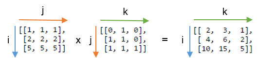
np.einsum('ij,jk->ik', A, B)
jjik
A = np.array([[1, 1, 1],
[2, 2, 2],
[5, 5, 5]])
B = np.array([[0, 1, 0],
[1, 1, 0],
[1, 1, 1]])
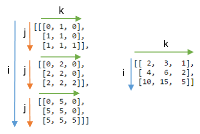
np.einsum('ij,jk->ijk', A, B)
A = np.array([[1, 1, 1],
              [2, 2, 2],
              [5, 5, 5]])

B = np.array([[0, 1, 0],
              [1, 1, 0],
              [1, 1, 1]])
C = np.einsum('ij,jk->ijk', A, B)
print(C, C.shape, sep='\n')
[[[0 1 0]
  [1 1 0]
  [1 1 1]]

 [[0 2 0]
  [2 2 0]
  [2 2 2]]

 [[0 5 0]
  [5 5 0]
  [5 5 5]]]
(3, 3, 3)
# C.sum(axis=1) # what happens if we do?
# np.einsum('ij,jk->ik', A, B)
A is $d\times 1$ and B is also $d\times 1$
| Call signature | NumPy equivalent | Description |
|---|---|---|
| ('i', A) | A | returns a view of A |
| ('i->', A) | sum(A) | sums the values of A |
| ('i,i->i', A, B) | A * B | element-wise multiplication of A and B |
| ('i,i', A, B) | inner(A, B) | inner product of A and B |
| ('i,j->ij', A, B) | outer(A, B) | outer product of A and B |
A is $i\times k$ and B is also $k\times j$
| Call signature | NumPy equivalent | Description |
|---|---|---|
| ('ij', A) | A | returns a view of A |
| ('ji', A) | A.T | view transpose of A |
| ('ii->i', A) | diag(A) | view main diagonal of A |
| ('ii', A) | trace(A) | sums main diagonal of A |
| ('ij->', A) | sum(A) | sums the values of A |
| ('ij->j', A) | sum(A, axis=0) | sum down the columns of A (across rows) |
| ('ij->i', A) | sum(A, axis=1) | sum horizontally along the rows of A |
| ('ij,ij->ij', A, B) | A * B | element-wise multiplication of A and B |
| ('ij,ji->ij', A, B) | A * B.T | element-wise multiplication of A and B.T |
| ('ij,jk', A, B) | dot(A, B) | matrix multiplication of A and B |
| ('ij,kj->ik', A, B) | inner(A, B) | inner product of A and B |
| ('ij,kj->ikj', A, B) | A[:, None] * B | each row of A multiplied by B |
| ('ij,kl->ijkl', A, B) | A[:, :, None, None] * B | each value of A multiplied by B |
C = np.einsum('ij,kl->ijkl', A, B)
C.shape
(3, 3, 3, 3)