Machine Learning

AI & Machine Learning - Unit 2

---

11. Backpropagation (Intro to Deep Learning)

Prof. Iacopo Masi - Computer Science Department, Sapienza University of Rome

Recap previous lecture

• Multi-Class Classification
• SoftMax Regression plus Cross-Entropy Loss
• Optimization in Deep Learing with SGD over mini-batch with momentum
• MLP and Fully-Connected Neural Nets
• Intro to Backpropagation

Today's lecture

Supervised, Parametric Models

Propaedeutic part for Deep Learning

0) Go back to Backpropagation

1) Backpropagation with matrices and vectors (Jacobians, Gradients)

2) End of the course! 🤖 🦿

This lecture material is taken from

• d2l.ai - Multi Variable Calculus
• Karpathy (Tesla Machine Learning Director) Lecture on Backprop
• Stanford Neural Nets and Backprop lecture
• Stanford ML notes on Neural Nets
• Stanford ML notes on Backprop
• Animation from jermwatt.github.io

Now you see why it's named Multi-Layer Perceptron (MLP)

Representation of a Single Layer

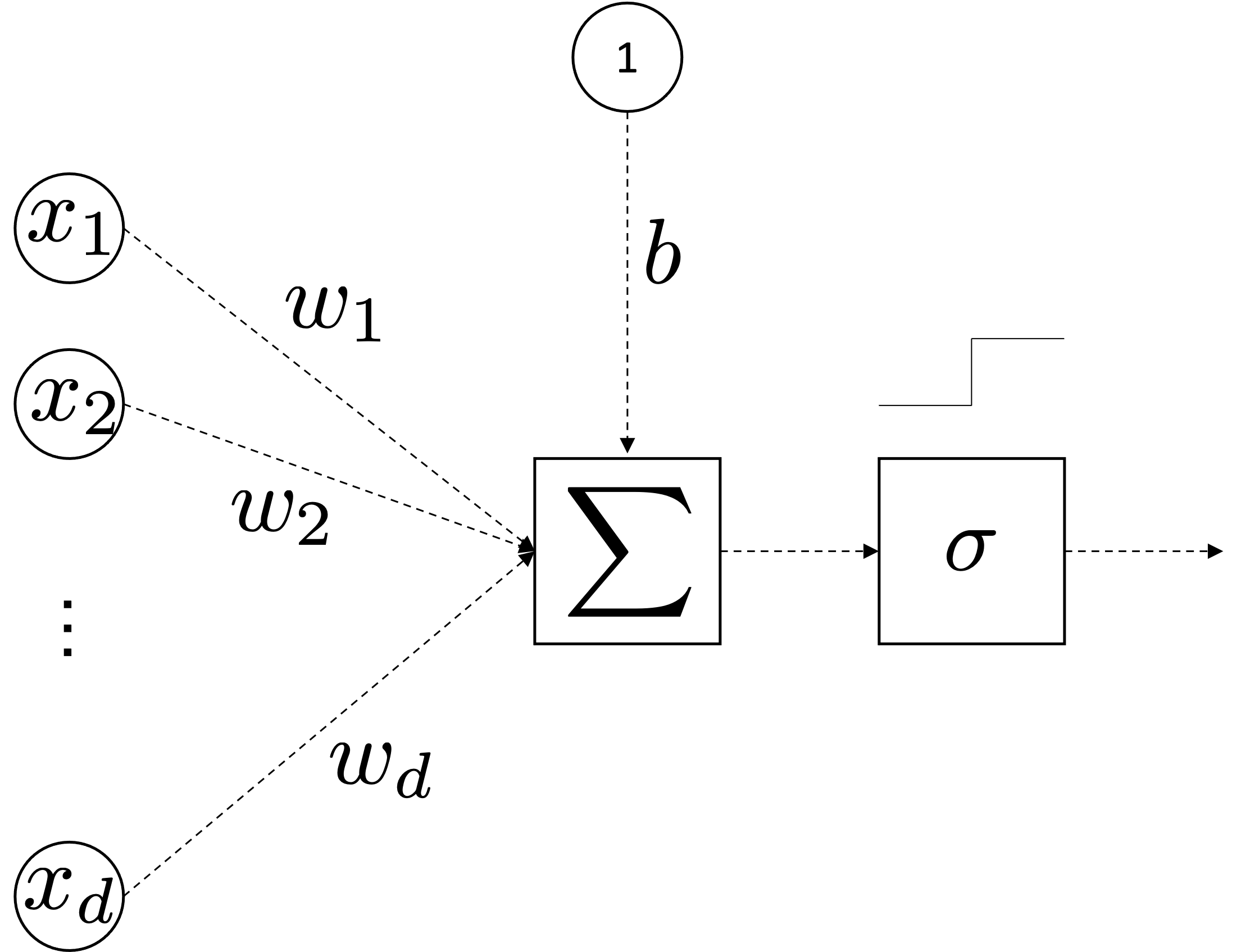
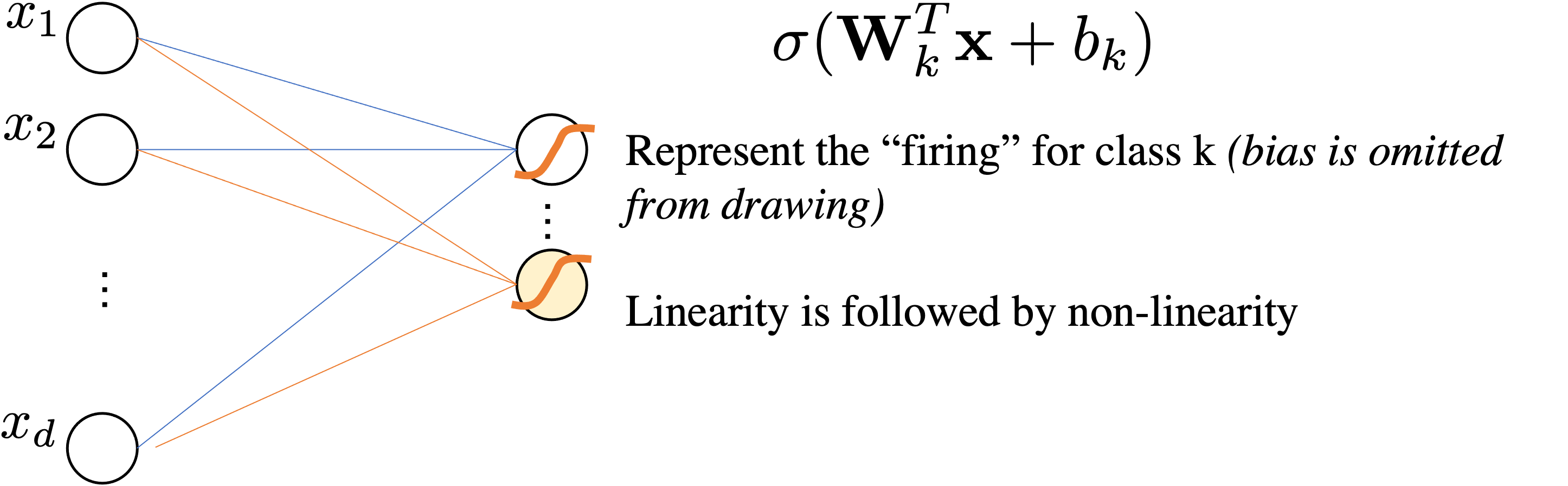
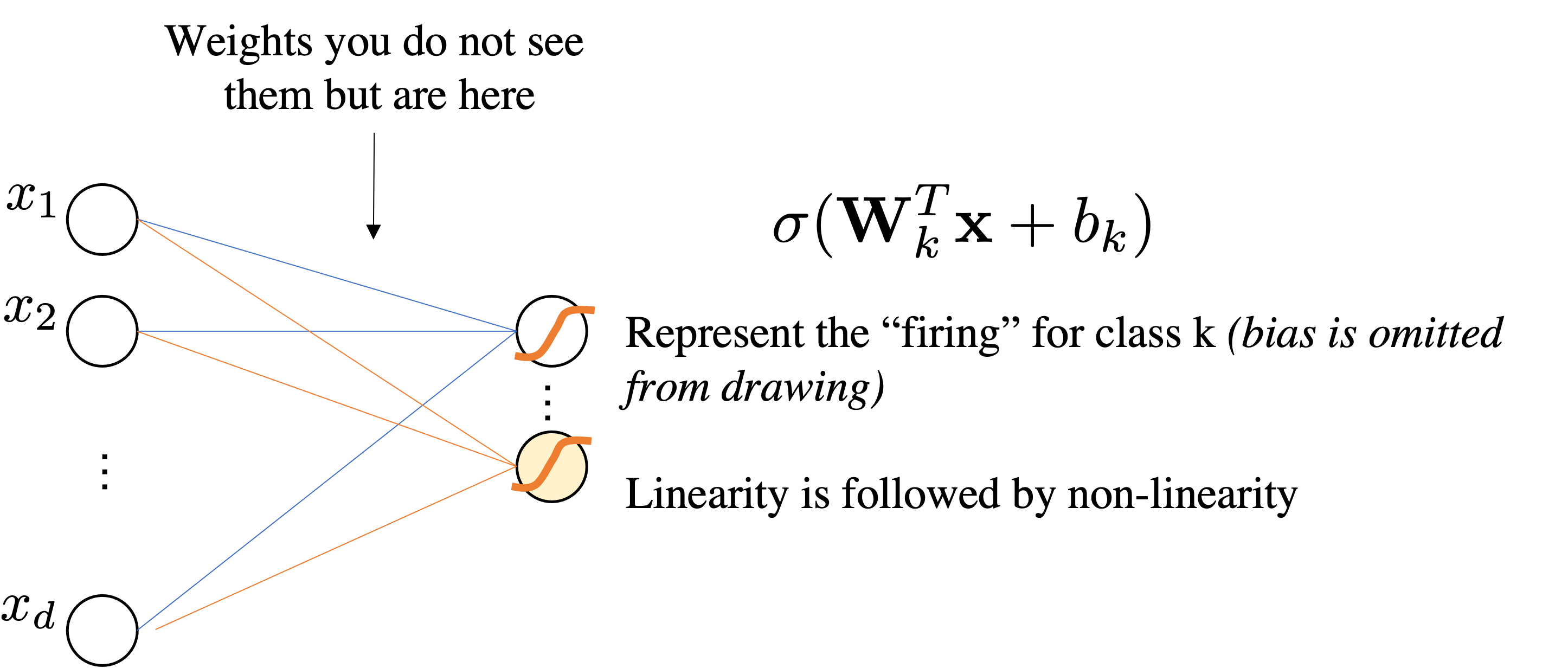
Let's consider our linear softmax regressor

$$ \underbrace{\mbf{z}}_{\mathbb{R}^{Kx1}} = \underbrace{\mbf{W}}_{\mathbb{R}^{K\times d}}\underbrace{\mbf{x}}_{\mathbb{R}^{d\times1}} + \underbrace{\mbf{b}}_{\mathbb{R}^K}$$

We interpret as Linear Layer $\mathbf{W} \mathbf{x}+\bmf{b}$ followed by Non-Linear Activation function $\sigma$

$$ \sigma(\mathbf{W} \mathbf{x} + \bmf{b})=\sigma \circ\left(\begin{array}{cccc} w_{11} & w_{12} & \cdots & w_{1 d} \\ w_{21} & w_{22} & \cdots & w_{2 d} \\ \vdots & \cdots & \ddots & \vdots \\ w_{k 1} & w_{m 2} & \cdots & w_{k d} \end{array}\right)\left(\begin{array}{c} x_{1} \\ x_{2} \\ \vdots \\ x_{d} \end{array}\right)+ \left(\begin{array}{c} b_{1} \\ b_{2} \\ \vdots \\ b_{k} \end{array}\right) =\sigma \circ\left(\begin{array}{c} z_{1} \\ z_{2} \\ \vdots \\ z_{k} \end{array}\right) $$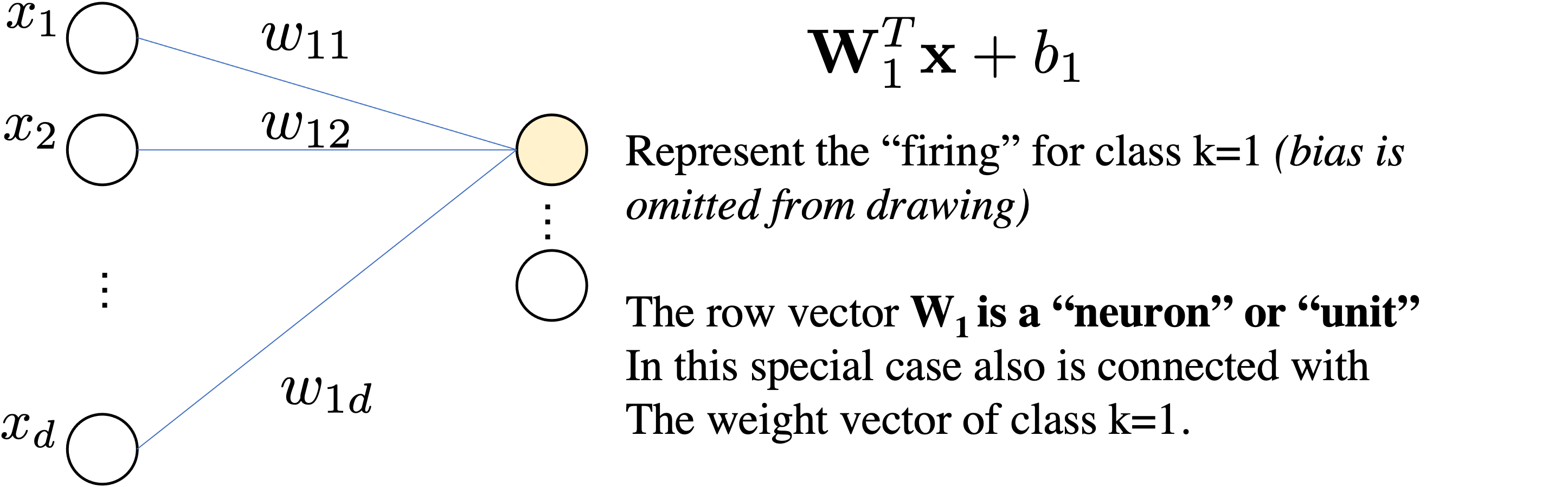

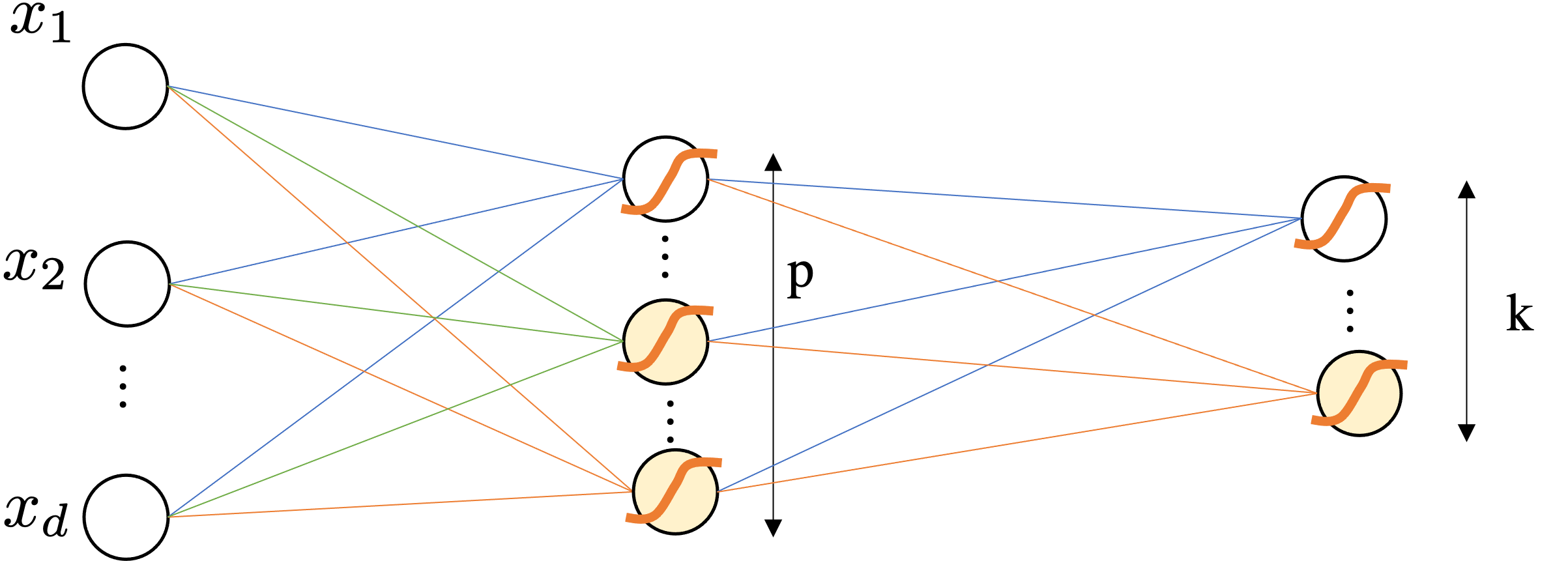
Representation of a Single Layer

$$ \sigma(\mathbf{W} \mathbf{x} + \bmf{b})=\sigma \circ\left(\begin{array}{cccc} \underline{w_{11}} & \underline{w_{12}} & \cdots & \underline{w_{1 d}} \\ w_{21} & w_{22} & \cdots & w_{2 d} \\ \vdots & \cdots & \ddots & \vdots \\ w_{k 1} & w_{m 2} & \cdots & w_{k d} \end{array}\right)\left(\begin{array}{c} x_{1} \\ x_{2} \\ \vdots \\ x_{d} \end{array}\right)+ \left(\begin{array}{c} b_{1} \\ b_{2} \\ \vdots \\ b_{k} \end{array}\right) =\sigma \circ\left(\begin{array}{c} z_{1} \\ z_{2} \\ \vdots \\ z_{k} \end{array}\right) $$

Representation of a Single Layer

$$ \sigma(\mathbf{W} \mathbf{x} + \bmf{b})=\sigma \circ\left(\begin{array}{cccc} {w_{11}} & {w_{12}} & \cdots & {w_{1 d}} \\ w_{21} & w_{22} & \cdots & w_{2 d} \\ \vdots & \cdots & \ddots & \vdots \\ \underline{w_{k 1}} & \underline{w_{m 2}} & \cdots & \underline{w_{k d}} \end{array}\right)\left(\begin{array}{c} x_{1} \\ x_{2} \\ \vdots \\ x_{d} \end{array}\right)+ \left(\begin{array}{c} b_{1} \\ b_{2} \\ \vdots \\ b_{k} \end{array}\right) =\sigma \circ\left(\begin{array}{c} z_{1} \\ z_{2} \\ \vdots \\ z_{k} \end{array}\right) $$

Representation of a Single Layer: Linear plus non-Linear

$$ \sigma(\mathbf{W} \mathbf{x} + \bmf{b})=\sigma \circ\left(\begin{array}{cccc} {w_{11}} & {w_{12}} & \cdots & {w_{1 d}} \\ w_{21} & w_{22} & \cdots & w_{2 d} \\ \vdots & \cdots & \ddots & \vdots \\ \underline{w_{k 1}} & \underline{w_{m 2}} & \cdots & \underline{w_{k d}} \end{array}\right)\left(\begin{array}{c} x_{1} \\ x_{2} \\ \vdots \\ x_{d} \end{array}\right)+ \left(\begin{array}{c} b_{1} \\ b_{2} \\ \vdots \\ b_{k} \end{array}\right) =\sigma \circ\left(\begin{array}{c} z_{1} \\ z_{2} \\ \vdots \\ z_{k} \end{array}\right) $$

Representation of a Single Layer: Linear plus non-Linear

$$ \mathbf{W} \mathbf{x}=\left(\begin{array}{c} -\text { unit - } \\ \vdots \\ -\text { unit }- \end{array}\right)\left(\begin{array}{c} \mid \\ \mathbf{x} \\ \mid \end{array}\right) $$

Representation as a computational graph

Adding another non-linear layer before the classifier

• We improve the expressiveness of our learned function by adding another NON-linear layer before the classification layer.
• Think this new layer as a feature map $\mbf{x} \mapsto \phi(\mbf{x})$; it maps our attribute to a feature space
• Now the classifier does not classify anymore directly $\mbf{x}$ but the feature $ \phi(\mbf{x})$.
• Sorry, notation becomes complex. Upper script means layer index; lower-script selects the unit
• $\mathbf{W}^1 \in \mathbb{R}^{d\times p}$, $\bmf{b}^1 \in \mathbb{R}^{p}$ so then $\mathbf{W}^2 \in \mathbb{R}^{p\times k}$, $\bmf{b}^2 \in \mathbb{R}^{k}$

$$\mbf{p}=\sigma(\mathbf{W}^2\underbrace{\left(\sigma(\mathbf{W}^1 \mathbf{x} + \bmf{b}^1) \right)}_{\bmf{\phi}(x)} + \bmf{b}^2)$$$$\text{dim. analysis:} \quad d \mapsto p \mapsto k$$

$\mathbf{W}^1 \in \mathbb{R}^{d\times p}$ is an Hidden Layer

Because it maps the original attribute in $d$ from an dimensionality $p$ and then $p$ is used for classifying.

A priori you do not know what $\mathbf{W}^1$ may learn.

$$\mbf{p}=\sigma(\mathbf{W}^2\underbrace{\left(\sigma(\mathbf{W}^1 \mathbf{x} + \bmf{b}^1) \right)}_{\bmf{\phi}(x)} + \bmf{b}^2)$$$$\text{dim. analysis:} \quad d \mapsto p \mapsto k$$

Let's update our visualizations

Multi-Layer Perceptron (MLP) with one hidden layer

Given the nature of these layers, they're called Fully-Connected NN

Multi-Layer Perceptron with one hidden layer

Non-linear activation functions: ReLu - Rectified Linear Unit

Very important: Activation Functions are computed element-wise.

$$ \sigma(z)= \max(0,z) \quad \text{ReLu}$$

ReLu is piece-wise linear function

Sigmoid

• Used to model output probability
• Nowadays not used in middle layers
• Have to compute $\exp()$
• Vanishing gradients for large input magnitude

ReLU

• Computationally efficient (no exp!)
• No vanishing gradients but do not let pass gradients for negative values
• Converge much faster than sigmoid (6x)
• Not differentiable in zero (subgradients)

Backpropagation and Differential Programming

NN can be huge composition of functions! 😱

Three ways of computing the gradients $\nabla_{\mbf{w}}\mathcal{L}(x,y;\mbf{w})$

1. Manually (if we change the network, we have to adjust it for a 100 layer neural net) maybe not a good idea, does not scale, even if we use symbolic derivation tools such as Mathematica ✍🏼
2. Finite Difference good to check the gradients once you have an automatic way of computing it; very slow, unfeasible in training! 👩🏾‍💻
3. Backpropagation: application of chain rule of calculus to tensors with a computational graph with caching (differential programming with automatic differentiation) 💻

1. Infeasible to derive manully the gradient update, let the machines work for us

2. Finite difference (very slow!) but used for gradient check

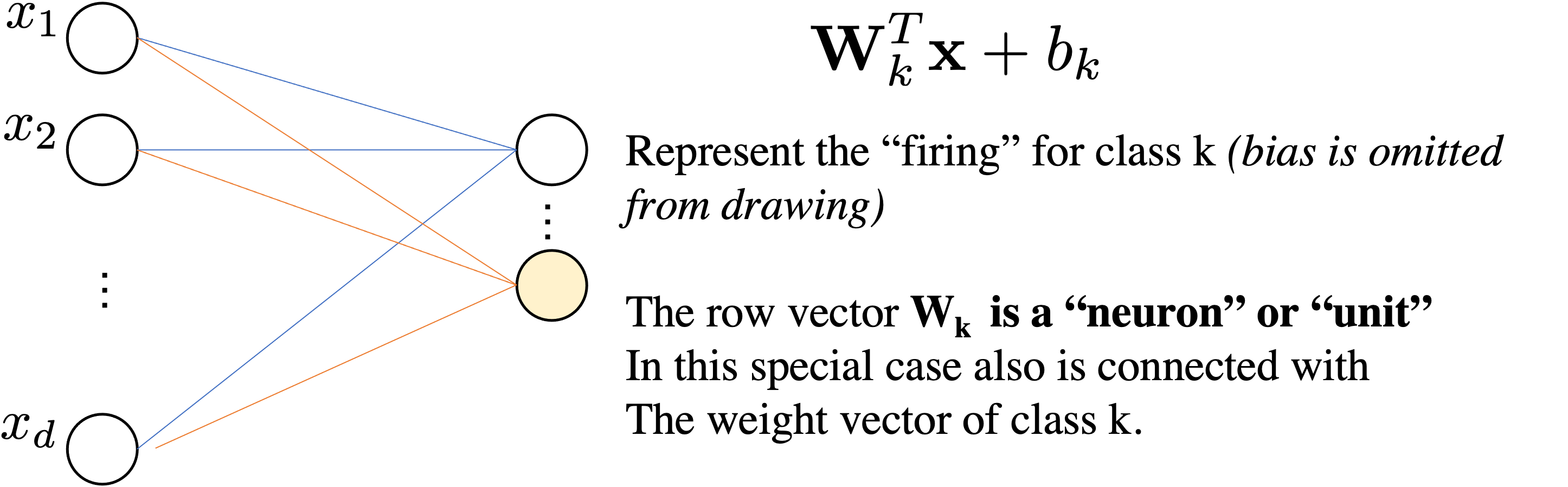
Assume $\mathbf{W}$ is your matrix and $w=\mathbf{W}_{ij}$ is a scalar inside your matrix.

• [Offline] Evaluate your NN loss at current weight value L(w)

For i,j=1....dims:

1. $w=\mathbf{W}_{ij}$
2. You want to see what is the impact of a paramter $w$ on the loss?
3. Perturb that $w$ by an $\epsilon=1e-5$ and evaluate the new loss at L(w+eps)
4. Numerical Gradient is [L(w+eps)-L(w)]/eps at position ij, so store it in $\nabla_{\mbf{W}}\mathcal{L}_{ij}$

$$\frac{\partial\mathcal{L}}{\partial w}(x,y;w)= \frac{L(w+\epsilon) - L(w)}{\epsilon}$$

At the end you have your numerical gradients $\nabla_{\mbf{W}}\mathcal{L}_{ij}$.

3. Backpropagation

Let's be clear on what we need to compute

$\forall l \in [1\ldots,L]$:

1. $\nabla_{\mbf{W}^l}\mathcal{L}(\mbf{x},y;\{\mbf{W},b\})$
2. $\nabla_{\mbf{b}^l}\mathcal{L}(\mbf{x},y;\{\mbf{W},b\})$
   
   

Once you have gradients on ALL weights $\implies$ We can update

$\forall l \in [1\ldots,L]$:

1. $\mbf{W}^l \leftarrow \mbf{W}^l - \gamma \nabla_{\mbf{W}^l}\mathcal{L}(\mbf{x},y;\{\mbf{W},b\})$
2. $\mbf{b}^l \leftarrow \mbf{b}^l - \gamma \nabla_{\mbf{b}^l}\mathcal{L}(\mbf{x},y;\{\mbf{W},b\})$
   
   

How do we get all the weights?

Mostly taken from here

Chain Rule

Returning to functions of a single variable, suppose that $y = f(g(x))$ and that the underlying functions $y=f(u)$ and $u=g(x)$ are both differentiable. The chain rule states that

$$\frac{dy}{dx} = \frac{dy}{du} \frac{du}{dx}.$$

What is the derivative of loss wrt x in the equation below? $$y = loss\big(g(h(i(x)))\big)$$

$$\frac{\partial loss}{\partial x} = \frac{\partial loss}{\partial g} \frac{\partial g}{\partial h}\frac{\partial h}{\partial i}\frac{\partial i}{\partial x}$$

Chain Rule on Directed Acyclic Graph (DAG)

Automate the computation of derivatives with computer science

1. Forward Pass
2. Backward Pass

Forward Pass

This is what we wanted: $$\frac{\partial\mathcal{L}}{\partial x},\frac{\partial\mathcal{L}}{\partial y},\frac{\partial\mathcal{L}}{\partial z}$$

Forward pass

1. Evaluate the function on input (the function is "hard-coded" with your model/code)
2. Store "local" derivative at each layer/gate

$$\frac{\partial\mathcal{L}}{\partial q}=z, \frac{\partial\mathcal{L}}{\partial z}=q, \frac{\partial\mathcal{q}}{\partial x}=1, \frac{\partial\mathcal{q}}{\partial y}=1$$

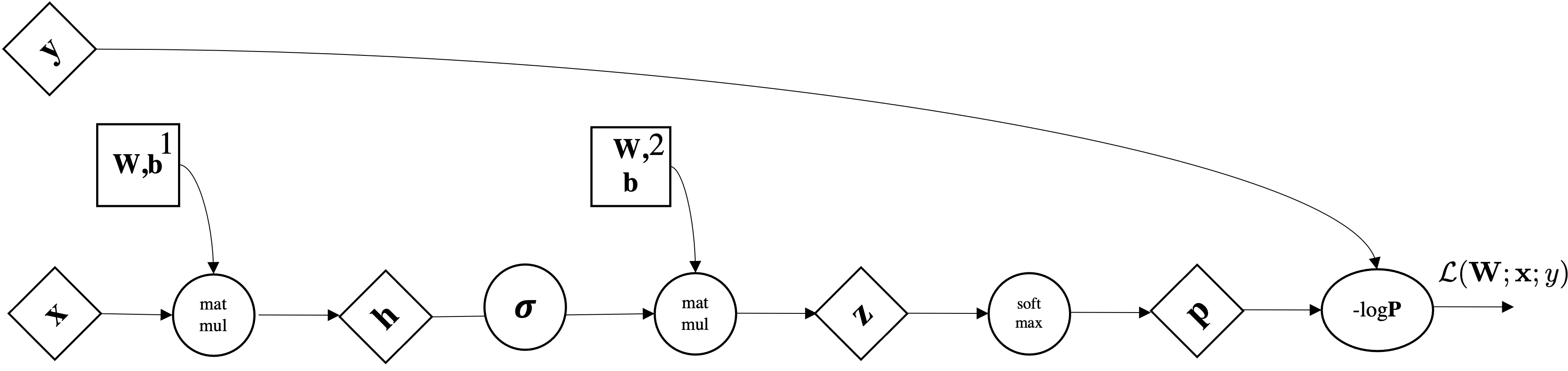
Backward Pass

What is the value of the gradient of $\mathcal{L}$ on $y$?: $$\frac{\partial\mathcal{L}}{\partial y} = \frac{\partial\mathcal{L}}{\partial q}\frac{\partial q}{\partial y} = z\cdot 1= -4$$

This is what we wanted: $$\frac{\partial\mathcal{L}}{\partial x},\frac{\partial\mathcal{L}}{\partial y},\frac{\partial\mathcal{L}}{\partial z}$$

Backward pass

1. Start from loss scalar value
2. Backpropagate the current derivative/gradient to higher layers
3. Use chain rule to aggregate a) local derivative b) what arrives from "the top"

$$\frac{\partial\mathcal{L}}{\partial q}=z, \frac{\partial\mathcal{L}}{\partial z}=q, \frac{\partial\mathcal{q}}{\partial x}=1, \frac{\partial\mathcal{q}}{\partial y}=1$$

Backward Pass

This is what we wanted: $$\frac{\partial\mathcal{L}}{\partial x},\frac{\partial\mathcal{L}}{\partial y},\frac{\partial\mathcal{L}}{\partial z}$$

This is what we have

$$\frac{\partial\mathcal{L}}{\partial q}=z, \frac{\partial\mathcal{L}}{\partial z}=q, \frac{\partial\mathcal{q}}{\partial x}=1, \frac{\partial\mathcal{q}}{\partial y}=1$$

Check with our manual derivation ✅

The high school way (as we did until now):

$$\frac{\partial\mathcal{L}(x,y,z)}{\partial x} = (\mbf{x}z+yz)^{\prime}=(\mbf{x}z)^{\prime}+(yz)^{\prime} = z = -4$$$$\frac{\partial\mathcal{L}(x,y,z)}{\partial y} = (xz+\mbf{y}z)^{\prime}=(xz)^{\prime}+(\mbf{y}z)^{\prime} = z = -4$$$$\frac{\partial\mathcal{L}(x,y,z)}{\partial z} = x+y = +3 $$

You know what? I do not trust math, I want to verify with a machine ✅

Pytorch check

from torch import tensor

def neural_net(x,y,z):
    return (x+y)*z

x, y, z = tensor(-2., requires_grad=True), tensor(5.,requires_grad=True), tensor(-4., requires_grad=True)
loss = neural_net(x,y,z) # forward pass
loss.backward()          # backward (after this I can check the gradients)
for el in [x,y,z]:
    print(el.grad)

tensor(-4.)
tensor(-4.)
tensor(3.)

Pytorch check

• Pytorch creates a dynamic computational directed acyclic graph (DAG) under the hood.

• We can also see the graph with Pytorch if you want (torchviz simplifies the plot)
• ! pip install torchviz

from torchviz import make_dot
from torch import tensor
def neural_net(x,y,z):
    return (x+y)*z

x, y, z = tensor(-2., requires_grad=True), tensor(5.,
                                                  requires_grad=True), tensor(-4., requires_grad=True)
loss = neural_net(x, y, z)  # forward pass

loss.backward()  # backward (ok now I can check the gradients)
for el in [x, y, z]:
    print(el.grad)
print(loss)
make_dot(loss, params=dict([('x', x),('y', y),('z', z)]))

tensor(-4.)
tensor(-4.)
tensor(3.)
tensor(-12., grad_fn=<MulBackward0>)

We can also see the DAG of AlexNet... [paper from 2012]

...but it won't fit my screen

import torch
from torchvision.models import AlexNet
model = AlexNet()
x = torch.randn(1, 3, 227, 227).requires_grad_(True)
y = model(x)
make_dot(y, params=dict(list(model.named_parameters()) + [('x', x)]))

General Recipe for Chain Rule over DAGs [Forward]

Just remember that you have to do at a generic gate:

General Recipe for Chain Rule over DAGs [Backward]

Multiply the gradient that you receive with your local gradient

Exam Question Lookalike

$$ f(w, x)=\frac{1}{1+e^{-\left(w_{0} x_{0}+w_{1} x_{1}+b\right)}} $$

Given the above function, can you perform forward and backward pass by writing all the local values and local gradient, by applying the chain rule?

(Direct computation of the gradient does not count for solving it, though you may be using it to double check)

Exam Question Lookalike [Forward Pass]

$$ f(w, x)=\frac{1}{1+e^{-\left(w_{0} x_{0}+w_{1} x_{1}+b\right)}} $$

Do not forget to store local gradients!

$$ f(w, x)=\frac{1}{1+e^{-\left(w_{0} x_{0}+w_{1} x_{1}+b\right)}} $$

Local gradients evaluated at input values! Now ready to go backwards

$$ f(w, x)=\frac{1}{1+e^{-\left(w_{0} x_{0}+w_{1} x_{1}+b\right)}} $$

End Forward; Now Ready to Backprop [Backward]

$$ f(w, x)=\frac{1}{1+e^{-\left(w_{0} x_{0}+w_{1} x_{1}+b\right)}} $$

End Forward; Now Ready to Backprop [Backward]

$$ f(w, x)=\frac{1}{1+e^{-\left(w_{0} x_{0}+w_{1} x_{1}+b\right)}} $$

End Forward; Now Ready to Backprop [Backward]

$$ f(w, x)=\frac{1}{1+e^{-\left(w_{0} x_{0}+w_{1} x_{1}+b\right)}} $$

End Forward; Now Ready to Backprop [Backward]

$$ f(w, x)=\frac{1}{1+e^{-\left(w_{0} x_{0}+w_{1} x_{1}+b\right)}} $$

End Forward; Now Ready to Backprop [Backward]

$$ f(w, x)=\frac{1}{1+e^{-\left(w_{0} x_{0}+w_{1} x_{1}+b\right)}} $$

End Forward; Now Ready to Backprop [Backward]

$$ f(w, x)=\frac{1}{1+e^{-\left(w_{0} x_{0}+w_{1} x_{1}+b\right)}} $$

End Forward; Now Ready to Backprop [Backward]

$$ f(w, x)=\frac{1}{1+e^{-\left(w_{0} x_{0}+w_{1} x_{1}+b\right)}} $$

End Backward

$$ f(w, x)=\frac{1}{1+e^{-\left(w_{0} x_{0}+w_{1} x_{1}+b\right)}} $$

Logistic Regression Computational Graph could be simplified

$$ f(w, x)=\frac{1}{1+e^{-\left(w_{0} x_{0}+w_{1} x_{1}+b\right)}} $$

This is what implements the Sigmoid Layer in Pytorch:

Logistic Regression Computational Graph could be simplified

$$ f(w, x)=\frac{1}{1+e^{-\left(w_{0} x_{0}+w_{1} x_{1}+b\right)}} $$

This is what implements the Sigmoid Layer in Pytorch:

Logistic Regression Computational Graph could be simplified

$$ f(w, x)=\frac{1}{1+e^{-\left(w_{0} x_{0}+w_{1} x_{1}+b\right)}} $$

This is what implements the Sigmoid Layer in Pytorch:

What PyTorch does very roughly [Pseudo code]

class ComputationalGraph:

    def forward(inputs):
        #1. pass inputs to input layers/gate
        #2. forward the computational graph
        for gate in self.graph.nodes_topologically_sorted():
            gate.forward()
        return loss # the finale gate outputs the loss

    def backward():
        for gate in reversed(self.graph.nodes_topologically_sorted()):
            gate.backward() # chain rule applied with local grads
        return inputs_grads

What is a Gate (ex. Multiplicative Scalar Gate) [Pseudo code]

class MultiplyGate:

    def forward(x,y):
        self.x = x # save local grads dz/dy
        self.y = y # save local grads dz/dx
        return x*y # eval function z = x + y

    def backward(dz):
        dx = self.y * dz # [dz/dx * dL/dz]
        dy = self.x * dz # [dz/dy * dL/dz]
        return [dx, dy]

Are we done with training neural nets?

Not completely: till now scalars, but we have matrices and vectors!

Now this looks more familiar

$\forall l \in [1\ldots,L]$:

1. $\mbf{W}^l \leftarrow \mbf{W}^l - \gamma \nabla_{\mbf{W}^l}\mathcal{L}(\mbf{x},y;\{\mbf{W},b\})$
2. $\mbf{b}^l \leftarrow \mbf{b}^l - \gamma \nabla_{\mbf{b}^l}\mathcal{L}(\mbf{x},y;\{\mbf{W},b\})$
   
   

Appendix: Gradient of Softmax wrt its probability

Gradient of SoftMax + CE Loss wrt $z$

\begin{split}\begin{aligned} \mathcal{L}(\mathbf{y}, \hat{\mathbf{y}}) &= - \sum_{j=1}^q y_j \log \frac{\exp(z_j)}{\sum_{k=1}^q \exp(z_k)} \\ &= \sum_{j=1}^q y_j \underbrace{\log \sum_{k=1}^q \exp(z_k)}_{\text{not vary with j = constant}} - \sum_{j=1}^q y_j z_j\\ &= \log \sum_{k=1}^q \exp(z_k) \quad \underbrace{\sum_{j=1}^q y_j}_{=1} \quad - \sum_{j=1}^q y_j z_j\\ &= \log \sum_{k=1}^q \exp(z_k) - \sum_{j=1}^q y_j z_j. \end{aligned}\end{split}

Taken from here

Gradient of SoftMax + CE Loss wrt $z$

Below we take the partial derivative wrt class j, so it is not in vector notation:

$$\partial_{z_j} \mathcal{L}(\mathbf{y}, \hat{\mathbf{y}}) = \frac{\exp(z_j)}{\sum_{k=1}^q \exp(z_k)} - y_j = \mathrm{softmax}(\mathbf{z})_j - y_j$$

It is a GLM!

Gradient of SoftMax + CE Loss wrt $z$

Below we take the partial derivative wrt class j, so it is not in vector notation:

$$\partial_{z_j} \mathcal{L}(\mathbf{y}, \hat{\mathbf{y}}) = \frac{\exp(z_j)}{\sum_{k=1}^q \exp(z_k)} - y_j = \mathrm{softmax}(\mathbf{z})_j - y_j$$

p = [0.2 0.7 0.1] y =[0 1 0]

dL/dz  = [0.2 (0.7-1) 0.1] = [0.2 -0.3 0.1]

Now this looks more familiar

$\forall l \in [1\ldots,L]$:

1. $\mbf{W}^l \leftarrow \mbf{W}^l - \gamma \nabla_{\mbf{W}^l}\mathcal{L}(\mbf{x},y;\{\mbf{W},b\})$
2. $\mbf{b}^l \leftarrow \mbf{b}^l - \gamma \nabla_{\mbf{b}^l}\mathcal{L}(\mbf{x},y;\{\mbf{W},b\})$

$$\chain{\mathcal{L}}{\mbf{W}^1} =~~?~~$$

$$\chain{\mathcal{L}}{\mbf{W}^1} = \chain{\loss}{\mbf{z}}\chain{\mbf{z}}{\mbf{W}^1}$$

Backprop

$$\chain{\mathcal{L}}{\mbf{W}^1} = \chain{\loss}{\mbf{z}}\chain{\mbf{z}}{\mbf{W}^1}$$

Backprop

$$\chain{\mathcal{L}}{\mbf{W}^1} = \chain{\loss}{\mbf{z}}\chain{\mbf{z}}{\mbf{W}^1}$$

Backprop

$$\chain{\mathcal{L}}{\mbf{W}^1} = \chain{\loss}{\mbf{z}}\chain{\mbf{z}}{\mbf{W}^1}$$$$\loss : \mbf{z} \mapsto \text{scalar} $$$$ \chain{\loss}{\mbf{z}} \in \mathbb{R}^{Z\times1}$$

Backprop

$$\chain{\mathcal{L}}{\mbf{W}^1} = \underbrace{\chain{\loss}{\mbf{z}}}_{\mathbb{R}^{1\times Z}}\underbrace{\chain{\mbf{z}}{\sigma}\chain{\mbf{\sigma}}{\mbf{W}^1}}_{\chain{\mbf{z}}{\mbf{W}^1}}$$

Backprop

$$\chain{\mathcal{L}}{\mbf{W}^1} = \underbrace{\chain{\loss}{\mbf{z}}}_{\mathbb{R}^{1\times Z}}\underbrace{\chain{\mbf{z}}{\sigma}\chain{\mbf{\sigma}}{\mbf{W}^1}}_{\chain{\mbf{z}}{\mbf{W}^1}}$$$$ \chain{\mbf{z}}{\mbf{\sigma}} =~~?~~$$

Backprop

$$\chain{\mathcal{L}}{\mbf{W}^1} = \underbrace{\chain{\loss}{\mbf{z}}}_{\mathbb{R}^{1\times Z}}\underbrace{\chain{\mbf{z}}{\sigma}\chain{\mbf{\sigma}}{\mbf{W}^1}}_{\chain{\mbf{z}}{\mbf{W}^1}}$$$$f : \mbf{\sigma} \mapsto \mbf{z} \quad \text{vector to vector}$$$$ \chain{\mbf{z}}{\mbf{\sigma}} =~~?~~; \mbf{z} = \mbf{W}\sigma+\mbf{b}$$

Backprop

$$\chain{\mathcal{L}}{\mbf{W}^1} = \underbrace{\chain{\loss}{\mbf{z}}}_{1\times Z}\underbrace{\chain{\mbf{z}}{\sigma}}_{Z\times \Sigma}\chain{\mbf{\sigma}}{\mbf{W}^1}$$$$f : \mbf{\sigma} \mapsto \mbf{z} \quad \text{vector to vector}$$$$ \chain{\mbf{z}}{\mbf{\sigma}} = \mbf{W}^{[2]}; \quad \mbf{z} = \mbf{W}^{[2]}\sigma+\mbf{b}^{[2]}$$

Backprop

$$\chain{\mathcal{L}}{\mbf{W}^1} = \underbrace{\chain{\loss}{\mbf{z}}}_{1\times Z}\underbrace{\chain{\mbf{z}}{\sigma}}_{Z\times \Sigma}\chain{\mbf{\sigma}}{\mbf{W}^1}$$$$f : \mbf{\sigma} \mapsto \mbf{z} \quad \text{vector to vector}$$$$ \chain{\mbf{z}}{\mbf{\sigma}} = \mbf{W}^{[2]}; \quad \mbf{z} = \mbf{W}^{[2]}\sigma+\mbf{b}^{[2]}$$

Backprop

$$\chain{\mathcal{L}}{\mbf{W}^1} = \underbrace{\chain{\loss}{\mbf{z}}}_{1\times Z}\underbrace{\chain{\mbf{z}}{\sigma}}_{Z\times \Sigma}\chain{\mbf{\sigma}}{\mbf{W}^1}$$$$f : \mbf{\sigma} \mapsto \mbf{z} \quad \text{vector to vector}$$$$ \chain{\mbf{z}}{\mbf{\sigma}} = \mbf{W}^{[2]}; \quad \mbf{z} = \mbf{W}^{[2]}\sigma+\mbf{b}^{[2]}$$

Backprop

$$\chain{\mathcal{L}}{\mbf{W}^1} = \underbrace{\chain{\loss}{\mbf{z}}}_{1\times Z}\underbrace{\chain{\mbf{z}}{\sigma}}_{Z\times \Sigma}\underbrace{\chain{\mbf{\sigma}}{\mbf{h}}\chain{\mbf{h}}{\mbf{W}^1}}_{\chain{\mbf{\sigma}}{\mbf{W}^1}}$$

Backprop

$$\chain{\mathcal{L}}{\mbf{W}^1} = \underbrace{\chain{\loss}{\mbf{z}}}_{1\times Z}\underbrace{\chain{\mbf{z}}{\sigma}}_{Z\times \Sigma}\underbrace{\chain{\mbf{\sigma}}{\mbf{h}}\chain{\mbf{h}}{\mbf{W}^1}}_{\chain{\mbf{\sigma}}{\mbf{W}^1}}$$$$f : \mbf{h} \mapsto \sigma \quad \text{vector to vector} \quad \text{- ReLU activation}$$$$ \chain{\mbf{\sigma}}{\mbf{h}} = ~?; \quad \mbf{h}_i = \max(0,\sigma_i) ~~\forall i \in 0\ldots\Sigma$$

Backprop

$$\chain{\mathcal{L}}{\mbf{W}^1} = \underbrace{\chain{\loss}{\mbf{z}}}_{1\times Z}\underbrace{\chain{\mbf{z}}{\sigma}}_{Z\times \Sigma}\underbrace{\chain{\mbf{\sigma}}{\mbf{h}}\chain{\mbf{h}}{\mbf{W}^1}}_{\chain{\mbf{\sigma}}{\mbf{W}^1}}$$$$f : \mbf{h} \mapsto \sigma \quad \text{vector to vector} \quad \textbf{- ReLU activation has a particular Jacobian};$$$$ \chain{\mbf{\sigma}}{\mbf{h}} = \operatorname{diag(\{0,1\}_{ii})}; \quad \mbf{h}_i = \max(0,\sigma_i) ~~\forall i$$

Backprop

$$\chain{\mathcal{L}}{\mbf{W}^1} = \underbrace{\chain{\loss}{\mbf{z}}}_{1\times Z}\underbrace{\chain{\mbf{z}}{\sigma}}_{Z\times \Sigma}\underbrace{\chain{\mbf{\sigma}}{\mbf{h}}\chain{\mbf{h}}{\mbf{W}^1}}_{\chain{\mbf{\sigma}}{\mbf{W}^1}}$$

Backprop

$$\chain{\mathcal{L}}{\mbf{W}^1} = \underbrace{\chain{\loss}{\mbf{z}}}_{1\times Z}\underbrace{\chain{\mbf{z}}{\sigma}}_{Z\times \Sigma}\underbrace{\chain{\mbf{\sigma}}{\mbf{h}}}_{\Sigma \times \Sigma}\chain{\mbf{h}}{\mbf{W}^1}$$

Jacobian of Activation Functions: implementation exploits sparse structure

• Jacobians for activation functions are full of zeros! Since they are diagonal matrix, they are not implemented as a full matrix in practice but as the diagonal vector.
• For a $2^{12}=4096$ input and $2^{12}=4096$ output with ReLU, the Jacobian would be of size $2^{24}=16M$!
• This would scale even worse if you think of a mini batch of 128 examples: $2^{12+7}=4096\cdot 128$. Jacobian of $2^{(12+7)2}=274B$!

Backprop

$$\chain{\mathcal{L}}{\mbf{W}^1} = \underbrace{\chain{\loss}{\mbf{z}}}_{1\times Z}\underbrace{\chain{\mbf{z}}{\sigma}}_{Z\times \Sigma}\underbrace{\chain{\mbf{\sigma}}{\mbf{h}}}_{\Sigma \times \Sigma}\chain{\mbf{h}}{\mbf{W}^1}$$

How to compute $\chain{\mbf{h}}{\mbf{W}^{[1]}}$ ? Matrix to vector function

Matrix notation (I dropped the layer number but $\mbf{W}$ is $\mbf{W}^{[1]}$): $$ \mbf{h} = \mbf{W}\mbf{x}+\mbf{b}$$

Vector Notation (slice a single row) let's consider the i-th row of $\mbf{h}$ so $h=\mbf{h}_i$:

$$ h = \mbf{w}^T\mbf{x}+b \quad \text{where } \mbf{w} \text{ selects i-th row of } \mbf{W}$$

Slice a single row

$$ h = \sum_j w_j x_j + b$$$$\chain{h}{w_j} = x_j$$

Gradient of $\mbf{h}$ wrt $\mbf{W}_{ij}$ ($\mbf{W}_{ij} \mapsto \mbf{h}$ )

$$ \mbf{h}_i = \sum_j \mbf{W}_{ij} x_j + \mbf{b}_i$$$$\chain{\mbf{h}}{\mbf{W}_{ij}} = \begin{bmatrix} 0\qquad \\ 0\qquad \\ \vdots\qquad \\ x_{j}~~i^{\text{th}} \text{row}\\ \vdots\qquad \\ 0\qquad \end{bmatrix}$$

Backprop $\loss$ to $\mbf{W}_{ij}^{[1]}$

$$\chain{\mathcal{L}}{\mbf{W}_{ij}^{[1]}} = \underbrace{\chain{\loss}{\mbf{z}}}_{1\times Z}\underbrace{\chain{\mbf{z}}{\sigma}}_{Z\times \Sigma~}\underbrace{\chain{\mbf{\sigma}}{\mbf{h}}}_{~\Sigma \times \Sigma}\underbrace{\chain{\mbf{h}}{\mbf{W}_{ij}^{[1]}}}_{~\Sigma\times 1}$$

Backprop $\loss$ to $\mbf{W}_{ij}^{[1]}$

Backprop $\loss$ to $\mbf{W}_{ij}^{[1]}$ simplified

Backprop $\loss$ to $\mbf{W}_{ij}^{[1]}$ simplified

Backprop $\loss$ to $\mbf{W}^{[1]}$

Once you have gradients on ALL weights $\implies$ We can update

$\forall l \in [1\ldots,L]$:

1. $\mbf{W}^l \leftarrow \mbf{W}^l - \gamma \nabla_{\mbf{W}^l}\mathcal{L}(\mbf{x},y;\{\mbf{W},b\})$
2. $\mbf{b}^l \leftarrow \mbf{b}^l - \gamma \nabla_{\mbf{b}^l}\mathcal{L}(\mbf{x},y;\{\mbf{W},b\})$
   
   

A look back to the Entire Course

AI & ML are interesting with striking applications but price to pay...

• Solid math background (probability, statistics, linear algebra, calculus)
• Computer scientist formulates/interprets math and knows what is best to turn it into computational system
• Have critical minds on how to evaluate ML systems

A look back to the Entire Course

A look back to the Entire Course

That's all folks! 👋🏼