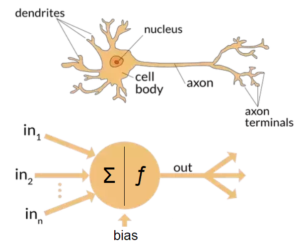
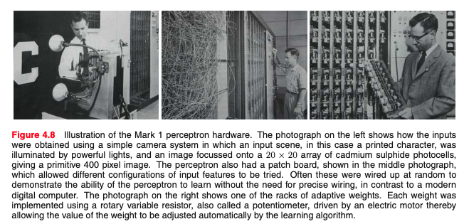
“Principles of Neurodynamics: Perceptrons and the Theory of Brain Mechanisms” published in 1962
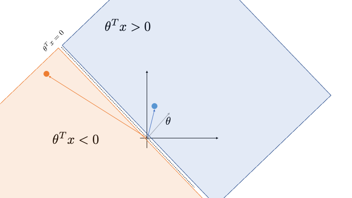
$\mbf{x}_i \in \mathbb{R}^d$ and $y \in \{0,1\}$
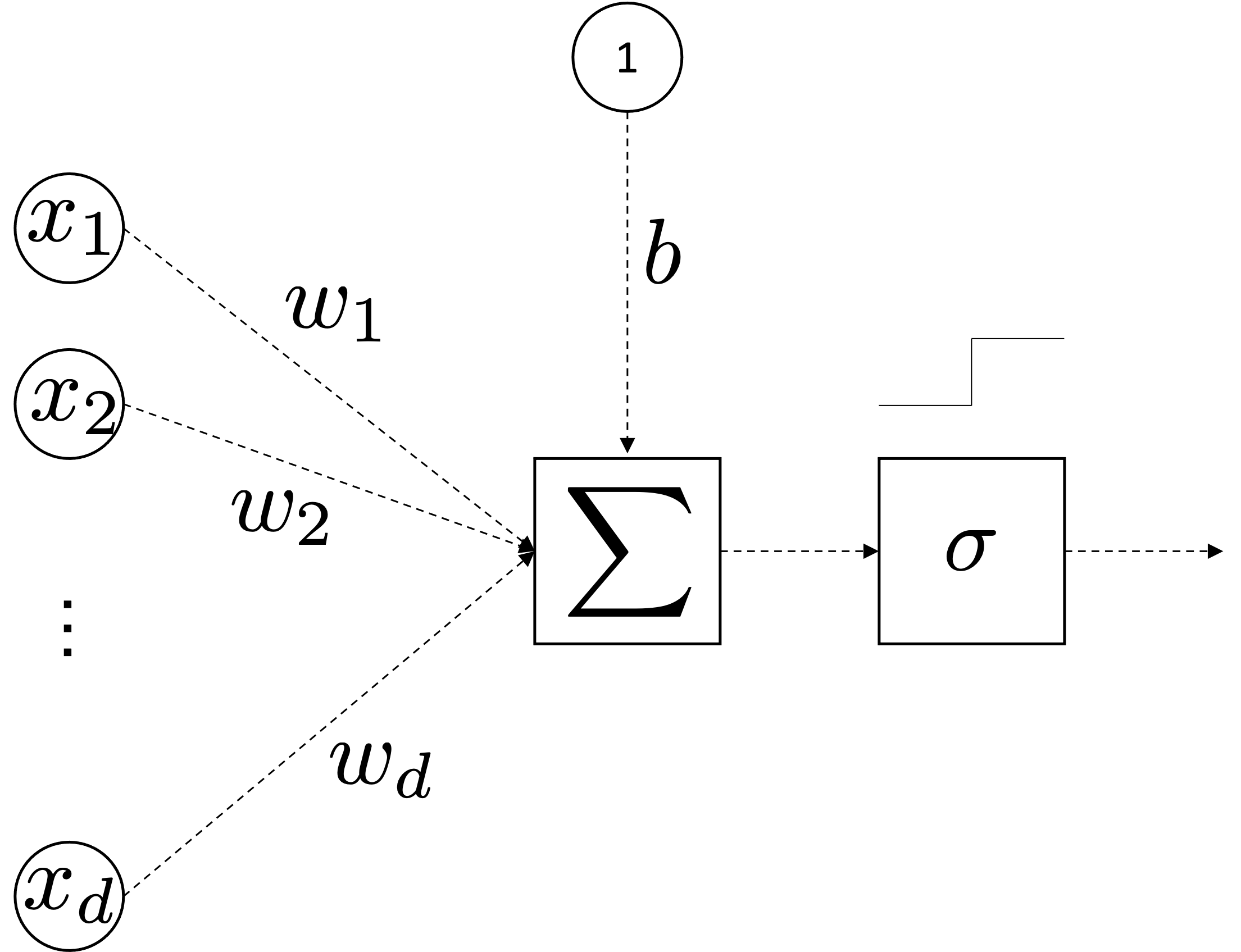
$$f_{\boldsymbol{\theta}}(\mbf{x}) \doteq \sigma\left( \bmf{\theta}^T\mbf{x} \right)$$where:
$$ \sigma(z)= \begin{cases} +1, & if& z\ge0 \\ 0, & if & z<0\end{cases}$$

A few observations:
A few observations:
A few observations:
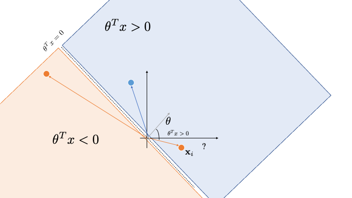
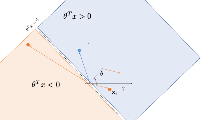

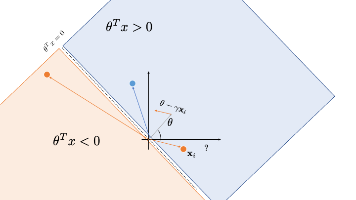
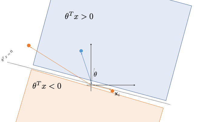
the angle is less than 90 deg, change $\theta \leftarrow \theta-\gamma\mbf{x}$the angle is more than 90 deg, change $\theta \leftarrow \theta+\gamma\mbf{x}$
the angle is less than 90 deg, change $\theta \leftarrow \theta-\gamma\mbf{x}$the angle is more than 90 deg, change $\theta \leftarrow \theta+\gamma\mbf{x}$
the angle is less than 90 deg, change $\theta \leftarrow \theta-\gamma\mbf{x}$the angle is more than 90 deg, change $\theta \leftarrow \theta+\gamma\mbf{x}$
$\theta$ is a linear combination of training samples $\{\mbf{x}_i,y_i\}$
Given a linearly separable training set, the Perceptron will find a generic solution of the infinite many that classifies correctly all the points (separate all the points neatly).
margin between points). Small margins require more time to converge.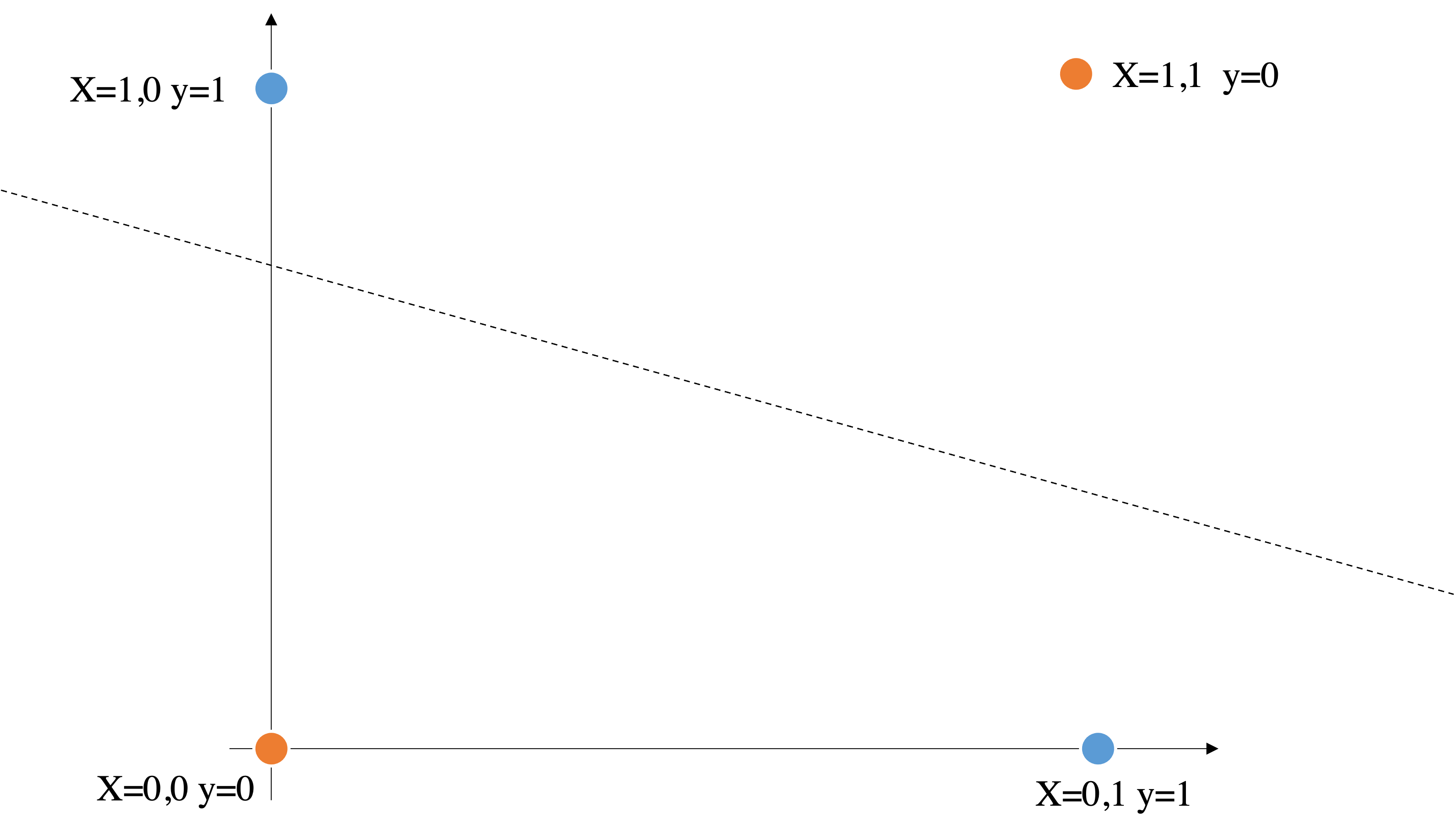
from sklearn.linear_model import Perceptron
from sklearn.preprocessing import PolynomialFeatures
import numpy as np

lift_features = True

X = np.array([[0, 0], [0, 1], [1, 0], [1, 1]])
y = X[:, 0] ^ X[:, 1]

if lift_features:
    print('X before=',X, sep='\n')
    X = PolynomialFeatures(interaction_only=True).fit_transform(X).astype(int)
    print('X before=',X,y.T, sep='\n')
clf = Perceptron(fit_intercept=False, max_iter=10, tol=None,
                 shuffle=False).fit(X, y)
clf.predict(X)
clf.score(X, y)
X before=
[[0 0]
 [0 1]
 [1 0]
 [1 1]]
X before=
[[1 0 0 0]
 [1 0 1 0]
 [1 1 0 0]
 [1 1 1 1]]
[0 1 1 0]
1.0
from sklearn.datasets import make_classification

X, y = make_classification(
    n_features=2, n_redundant=0, n_informative=2,
    n_clusters_per_class=1, random_state=0, class_sep=2.8)
plt.scatter(*X.T,c=y,cmap='jet');

from sklearn.datasets import make_classification
from matplotlib import cm
from celluloid import Camera
from IPython.display import HTML

def get_support(minx, maxx):
    support = np.linspace(minx, maxx, 100)
    xx, yy = np.meshgrid(support, support)
    points = np.stack((xx.flatten(), yy.flatten()), axis=1)
    points = add_ones(points)
    return points, xx, yy

def plot_separating_plane(w, minx, maxx, points, xx, yy):
    dist = perceptron(w, points.T)
    dist = dist.reshape(xx.shape)
    plt.contourf(xx, yy, dist, cmap=cm.get_cmap("RdBu"))
    plt.plot(0, 0, 'rx')
    plt.axis('scaled')
    plt.xlim(minx, maxx)


def perceptron(w, xi):
    return np.maximum(np.sign(np.dot(w, xi)), 0)


def add_ones(X):
    bias = np.ones((X.shape[0], 1))
    X = np.hstack((X, bias))
    return X

def done(w, X):
    return np.all(y == perceptron(w, X.T))


def plot_classification(theta_curr, minx, maxx, support, xx, yy, X):
    plot_separating_plane(theta_curr, minx, maxx, support, xx, yy)
    plt.scatter(X[:, 0], X[:, 1], s=80,c=y,
            facecolors="none",
            zorder=10,
            edgecolors="k",
            cmap=cm.get_cmap("RdBu"))

### CAMERA ##########
fig = plt.figure()
camera = Camera(fig)

################## DATA #####################
#X, y = make_classification(
#    n_features=2, n_redundant=0, n_informative=2,
#    n_clusters_per_class=1,
#    random_state=0, class_sep=2.8)
minx, maxx = X.min(), X.max()
support, xx, yy = get_support(minx, maxx)
X = add_ones(X)
############### PARAMS ########################
theta_curr = np.array([[-1, -2, 0]])
gamma = 1e-2
i = 0
text_kwargs = dict(ha='center', va='center', fontsize=10, color='C1')
################################################
plot_separating_plane(theta_curr, minx, maxx, support, xx, yy)
exit = False
# while not all are classified
while not done(theta_curr,X) and i < 300:
    # for all points
    for xi, yi in zip(X, y):
        prediction = perceptron(theta_curr, xi)
        # if prediction is wrong, update
        if prediction != yi:
            diff = yi - perceptron(theta_curr, xi)
            theta_curr = theta_curr + gamma * diff * xi
            plot_classification(theta_curr, minx, maxx, support, xx, yy, X)
            i += 1
            plt.text(-4, 4.5, str(i), **text_kwargs)
            camera.snap()
# write 20 frames with the last result for memory
for i in range(20):
    plot_classification(theta_curr, minx, maxx, support, xx, yy, X)
    camera.snap()
animation = camera.animate()
HTML(animation.to_html5_video())

where:
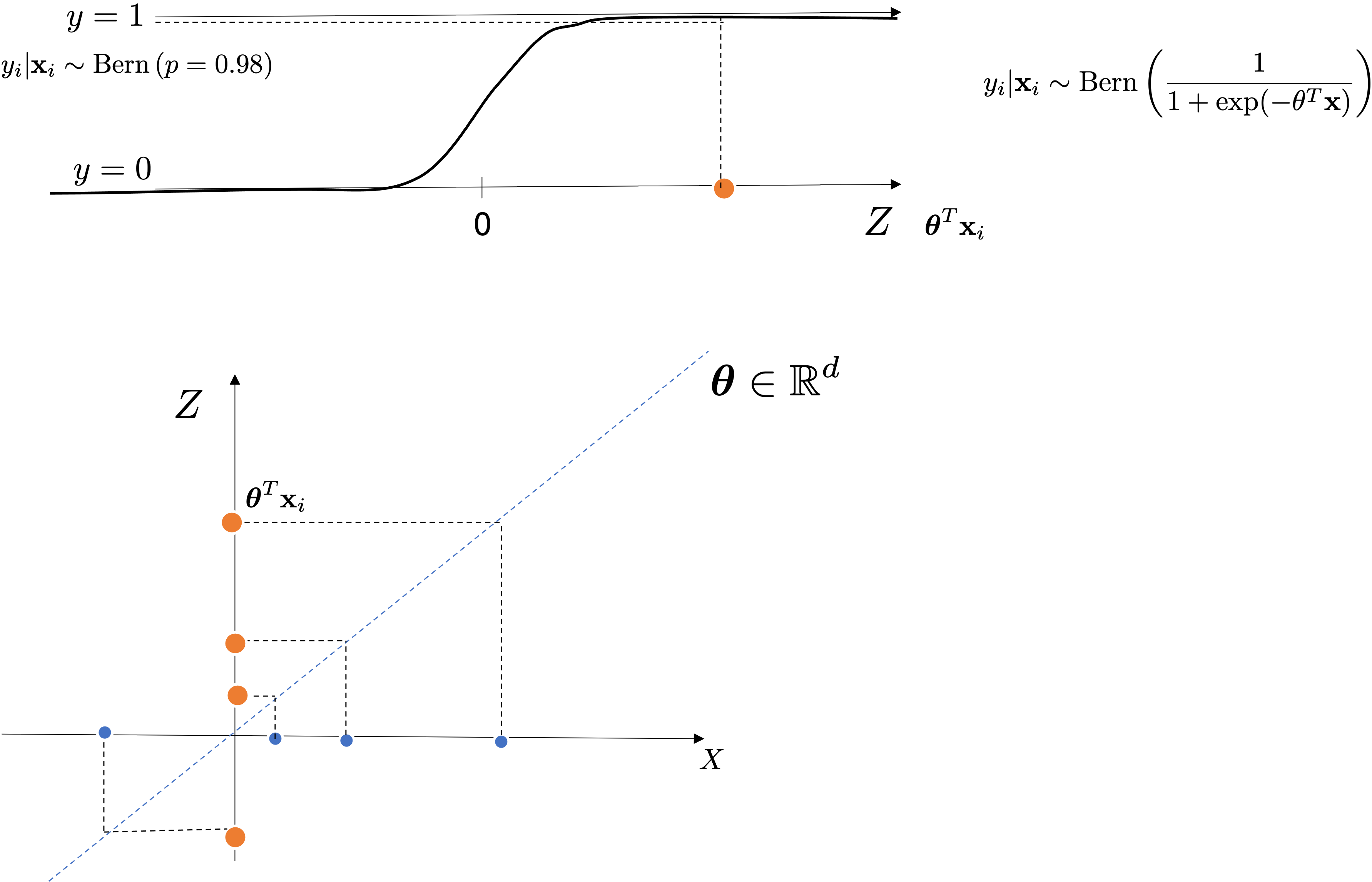
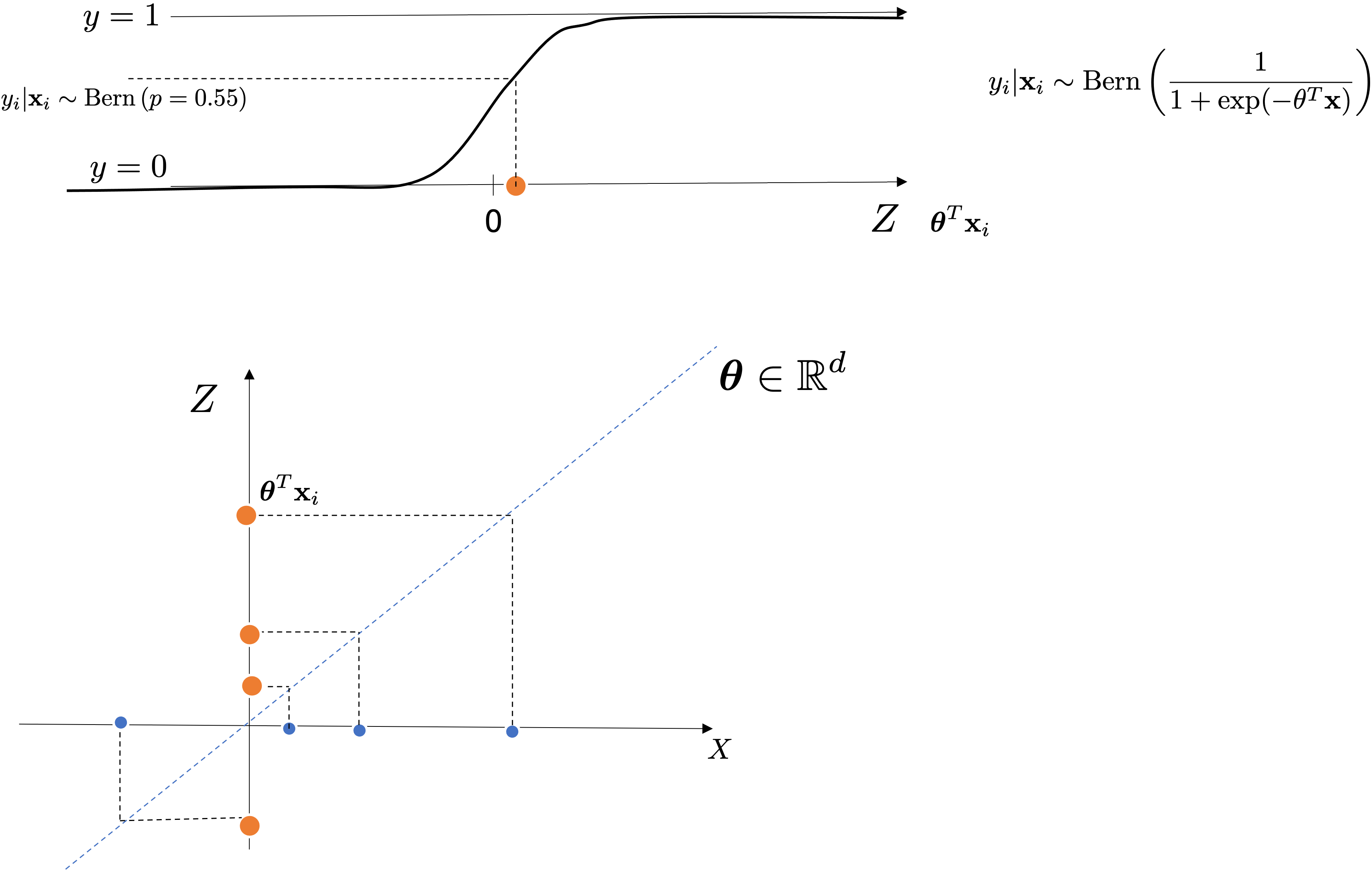
$$ \sigma(z)= \frac{1}{1+\exp^{-z}} \quad \text{sigmoid or logistic function}$$

We model conditional probability of $y|x$:
$$ \begin{cases} p(y=1| \mbf{x};\bmf{\theta}) = f_{\boldsymbol{\theta}}\\ p(y=0| \mbf{x};\bmf{\theta}) = ?\\ \end{cases} $$
$$f_{\boldsymbol{\theta}}(\mbf{x}) \doteq \sigma\left( \bmf{\theta}^T\mbf{x} \right)$$
where:
$$ \sigma(z)= \frac{1}{1+\exp^{-z}} \quad \text{sigmoid or logistic function}$$We model conditional probability of $y|x$:
$$ \begin{cases} p(y=1| \mbf{x};\bmf{\theta}) = f_{\boldsymbol{\theta}}\\ p(y=0| \mbf{x};\bmf{\theta}) = 1- f_{\boldsymbol{\theta}}\ \end{cases} $$
$$f_{\boldsymbol{\theta}}(\mbf{x}) \doteq \sigma\left( \bmf{\theta}^T\mbf{x} \right)$$
where:
$$ \sigma(z)= \frac{1}{1+\exp^{-z}} \quad \text{sigmoid or logistic function}$$$$\lim_{z\mapsto \infty}\sigma(z)=1$$$$\lim_{z\mapsto -\infty}\sigma(z)=0$$We model conditional probability of $y|x$:
$$ \begin{cases} p(y=1| \mbf{x};\bmf{\theta}) = f_{\boldsymbol{\theta}}\\ p(y=0| \mbf{x};\bmf{\theta}) = 1- f_{\boldsymbol{\theta}}\ \end{cases} $$
$$f_{\boldsymbol{\theta}}(\mbf{x}) \doteq \frac{1}{1+\exp^{-\bmf{\theta}^T\mbf{x}}}$$
import numpy as np;
import matplotlib.pyplot as plt;
x = np.arange(-20.0, 20.0, 0.1);
ws = np.array([0, 0.01,0.1,0.5,1,2,10,30])
for w in ws:
    y = 1/(1+np.exp(-w*x));
    plt.plot(x,y);
plt.legend(ws);

import numpy as np;
import matplotlib.pyplot as plt;
x = np.arange(-20.0, 20.0, 0.1);
ws = np.array([0, 0.01,0.1,0.5,1,2,10,30])*-1
for w in ws:
    y = 1/(1+np.exp(-w*x));
    plt.plot(x,y);
plt.legend(ws);

Points on the decision boundary: $~~~\bmf{\theta}^T\mbf{x}=0$
$$f_{\boldsymbol{\theta}}(\mbf{x}) \doteq \frac{1}{1+\exp^{-\bmf{\theta}^T\mbf{x}}} = \frac{1}{1+\exp^{0}} = \frac{1}{1+1}=\frac{1}{2}$$import numpy as np;import matplotlib.pyplot as plt;x = np.arange(-20.0, 20.0, 0.1);y = 1/(1+np.exp(-x));plt.plot(x,y);plt.plot(x,1-y);_=plt.legend(['p(y=1|x)','p(y=0|x)'])

In general the threshold is 0.5 to map it to a predicted class.
$$\frac{1}{1+\exp^{-\bmf{\theta}^T\mbf{x}}} > 0.5$$import numpy as np;import matplotlib.pyplot as plt;x = np.arange(-20.0, 20.0, 0.1);y = 1/(1+np.exp(-x));plt.plot(x,y);plt.plot(x,1-y);_=plt.legend(['p(y=1|x)','p(y=0|x)'])
We model conditional probability of $y|x$:
$$ \begin{cases} p(y=1| \mbf{x};\bmf{\theta}) = f_{\boldsymbol{\theta}}\\ p(y=0| \mbf{x};\bmf{\theta}) = 1- f_{\boldsymbol{\theta}}\\ \end{cases} $$For a single point, the if else above based on the $y$ can be written compactly as:
Which discrete distribution does the equation above resemble?
| Data Type $y$ | Expo. Family | Name/ML Topic |
|---|---|---|
| $\mathbb{R}$ | Gaussian LaPlace |
Regression |
| $\{0,1\}$ | Bernoulli | Binary Classification |
| $\{1,K\}$ | Categorical | Multi-class Classification |
| $\mathbb{N}_{+}$ | Poisson | Poisson Regression (Counts) |
| Categorical | Dirichlet | More advanced Topics |
Property of GLM
| Data Type $y$ | Expo. Family | Name |
|---|---|---|
| $\mathbb{R}$ | Gaussian LaPlace |
Regression |
| $\{0,1\}$ | Bernoulli | Binary Classification |
| $\{1,K\}$ | Categorical | Multi-class Classification |
| $\mathbb{N}_{+}$ | Poisson | Poisson Regression |
| Categorical | Dirichlet | More advanced Topics |
| Data Type $y$ | Expo. Family | Name |
|---|---|---|
| $\mathbb{R}$ | Gaussian LaPlace |
Regression |
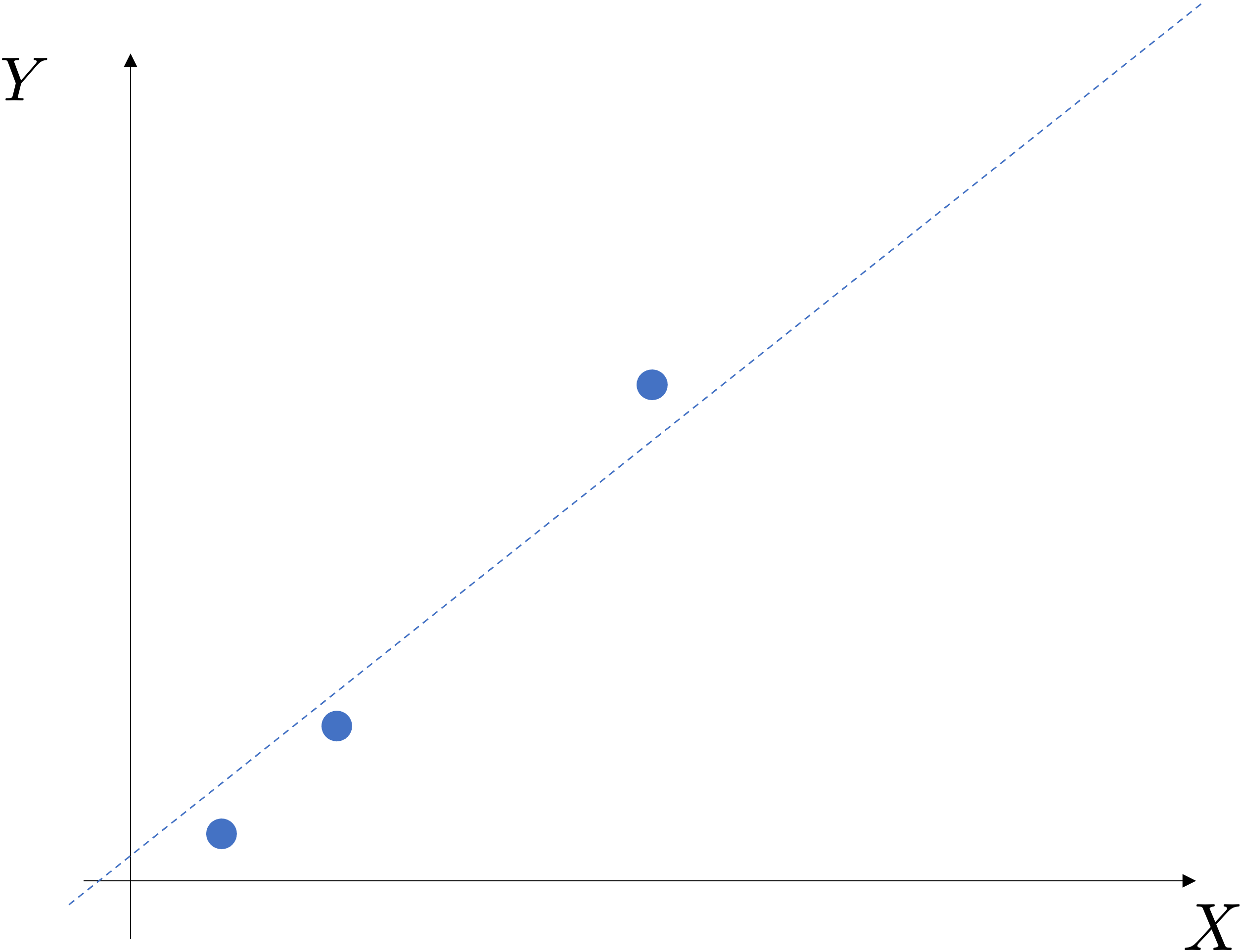
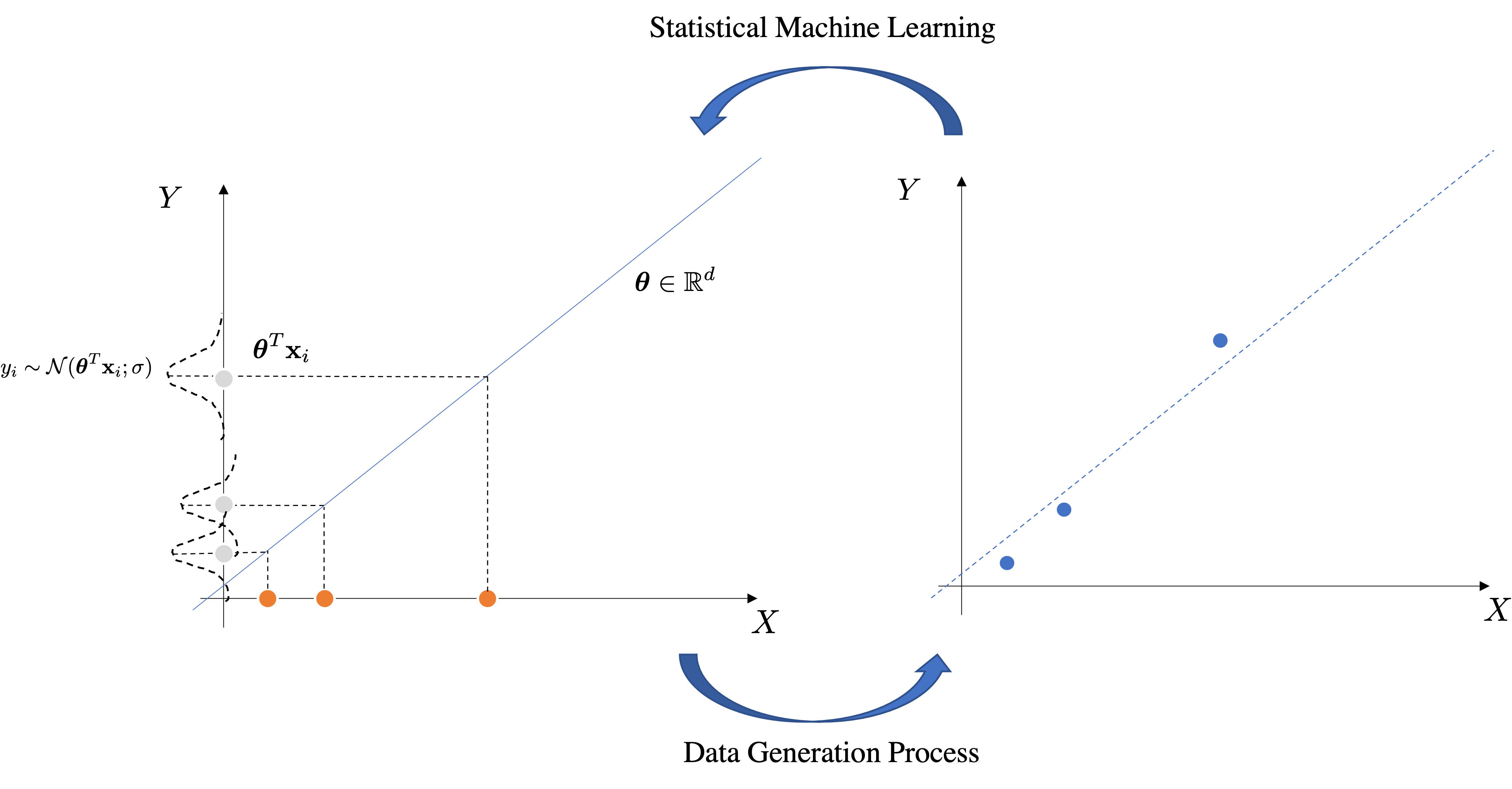
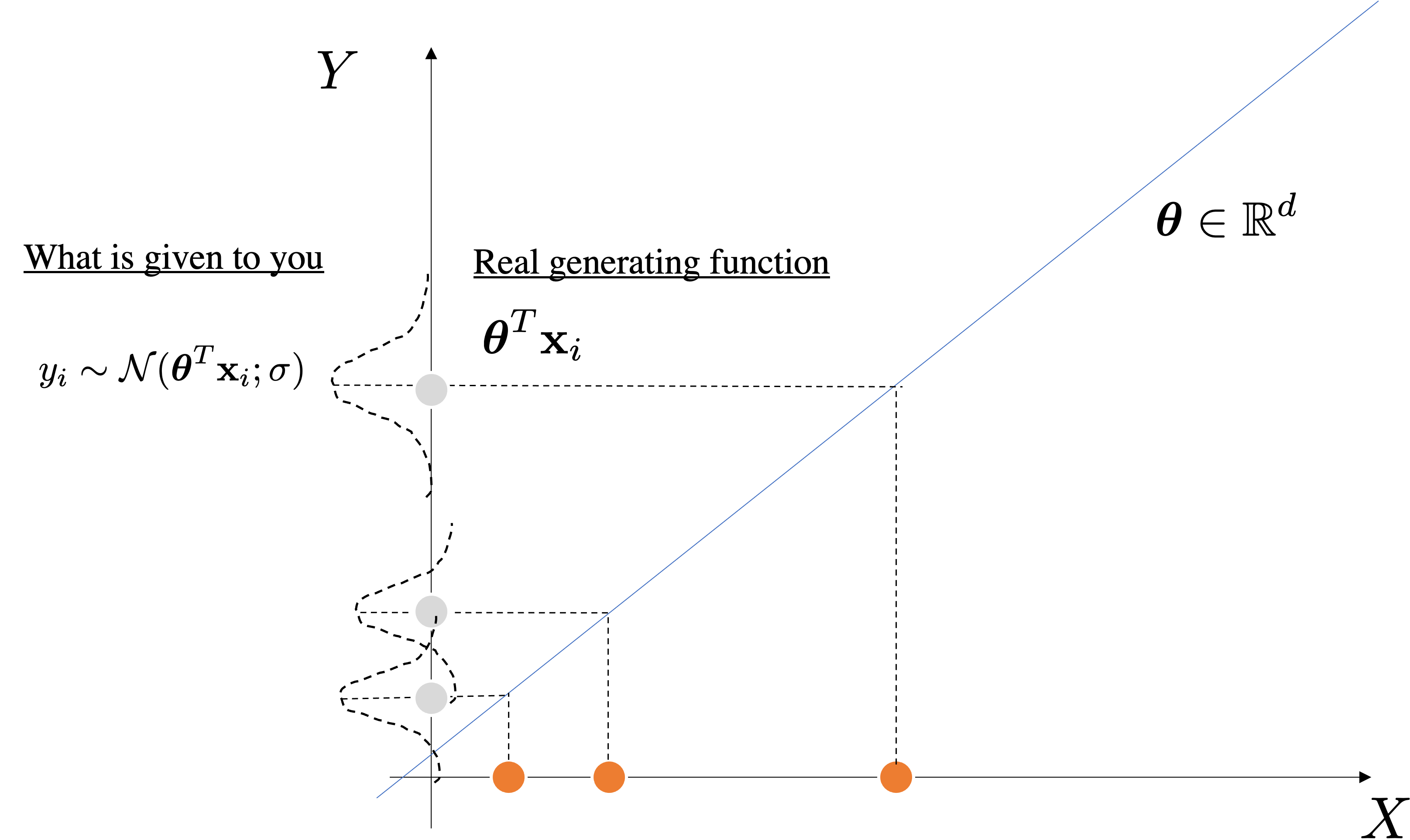
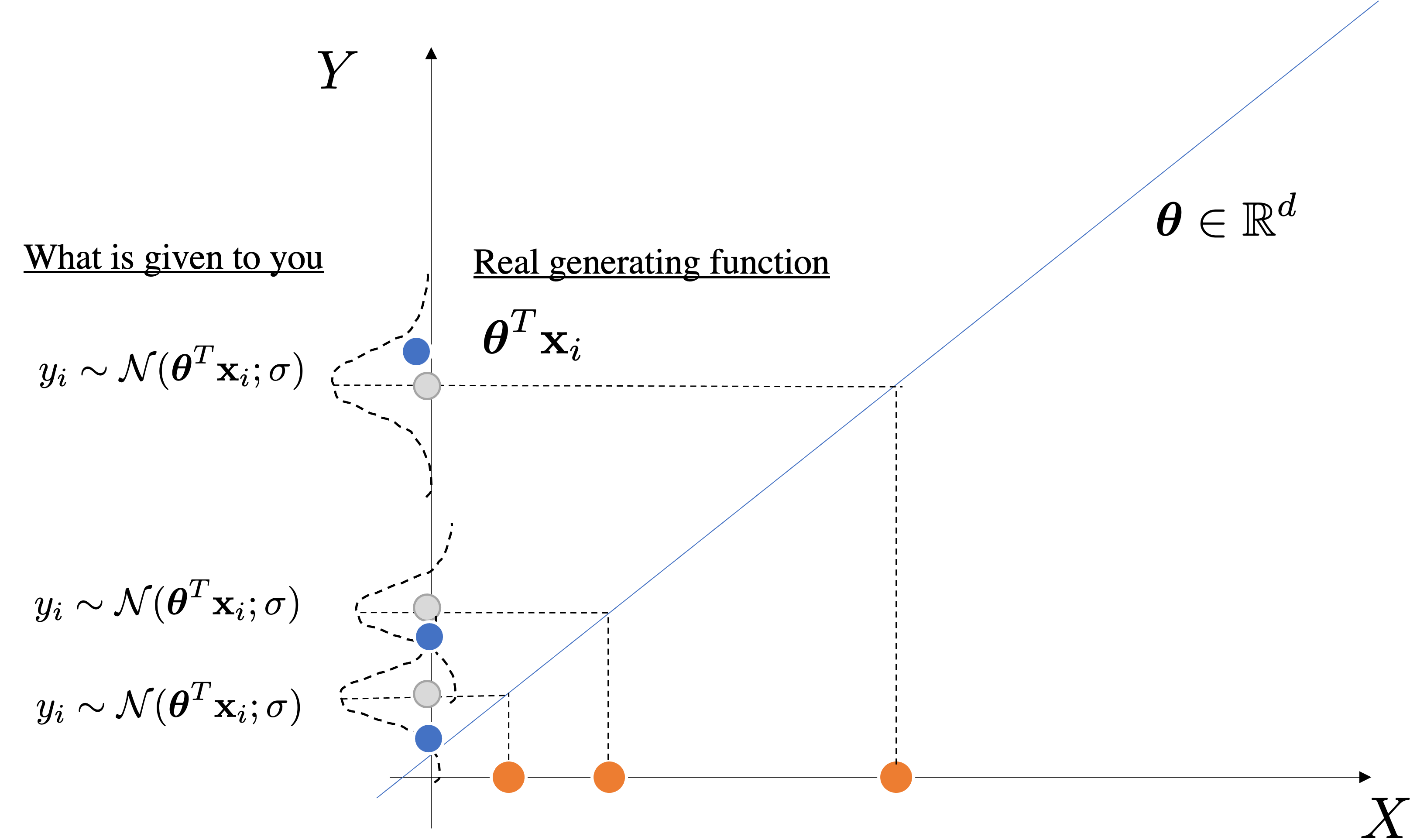
Generation process: $$ y = \mathcal{N}(\bmf{\theta}^T\mbf{x};\sigma^2)~~ \text{same as }~~ y = \theta^T\mbf{x} + \epsilon~~\text{with}~~\epsilon \sim \mathcal{N}(0;\sigma^2)$$
Generation process: $$ y = \mathcal{N}(\bmf{\theta}^T\mbf{x};\sigma^2)~~ \text{same as }~~ y = \theta^T\mbf{x} + \epsilon~~\text{with}~~\epsilon \sim \mathcal{N}(0;\sigma^2)$$
Generation process: $$ y = \mathcal{N}(\bmf{\theta}^T\mbf{x};\sigma^2)~~ \text{same as }~~ y = \theta^T\mbf{x} + \epsilon~~\text{with}~~\epsilon \sim \mathcal{N}(0;\sigma^2)$$
We model conditional probability of $y|x$:
$$ \begin{cases} p(y=1| \mbf{x};\bmf{\theta}) = f_{\boldsymbol{\theta}}\\ p(y=0| \mbf{x};\bmf{\theta}) = 1- f_{\boldsymbol{\theta}}\ \end{cases} $$For multiple training points, using I.I.D. assumptions:
$$ \begin{aligned} L(\theta;\mbf{X};\mbf{y}) &=p(\vec{y} \mid X ; \theta) =\\ L(\theta;\mbf{X};\mbf{y}) &=p(\vec{y} \mid {\mbf{x}_1,\ldots,\mbf{x}_n} ; \theta)= [IID] \\ &=\prod_{i=1}^{n} p\left(y^{(i)} \mid x^{(i)} ; \theta\right) \\ &=\prod_{i=1}^{n}\left(f_{\boldsymbol{\theta}}\left(x^{(i)}\right)\right)^{y^{(i)}}\left(1-f_{\boldsymbol{\theta}}\left(x^{(i)}\right)\right)^{1-y^{(i)}} \end{aligned} $$We get the Log-loss that we have seen in the lecture on evaluating the models!
$$
\begin{aligned}
\ell(\theta) &=\log L(\theta) \\
&=\sum_{i=1}^{n} y^{(i)} \log f\left(x^{(i)}\right)+\left(1-y^{(i)}\right) \log \left(1-f\left(x^{(i)}\right)\right)
\end{aligned}
$$
We get the Log-loss that we have seen in the lecture on evaluating the models!
$$ \begin{aligned} &\nabla_{\theta}\log L(\theta)= \\ &=\nabla_{\theta}\sum_{i=1}^{n} y^{(i)} \log f_{\theta}\left(x^{(i)}\right)+\left(1-y^{(i)}\right) \log \left(1-f_{\theta}\left(x^{(i)}\right)\right) \end{aligned} $$but before let's compute the gradient of the logistic function.
We get the Log-loss that we have seen in the lecture on evaluating the models!
$$ \begin{aligned} &\nabla_{\theta}\log L(\theta)= \\ &=\nabla_{\theta}\sum_{i=1}^{n} y^{(i)} \log f_{\theta}\left(x^{(i)}\right)+\left(1-y^{(i)}\right) \log \left(1-f_{\theta}\left(x^{(i)}\right)\right) \end{aligned} $$We get the Log-loss that we have seen in the lecture on evaluating the models!
$$ \begin{aligned} &\nabla_{\theta}\log L(\theta)= \\ &=\nabla_{\theta}\sum_{i=1}^{n} y^{(i)} \log[\sigma{(\theta^Tx^{(i)})}]+\left(1-y^{(i)}\right) \log [1-\sigma{(\theta^Tx^{(i)})}] \end{aligned} $$Remember:
$$\sigma(z)' = \sigma(z)(1-\sigma(z)) $$All latest parametric supervised problems we have discussed are convex.
The loss in function of the parameters is convex.
GD gives you a global minimum/maximum on convex functions (optimization is easy)
# Generate a toy dataset, it's just a straight line with some Gaussian noise:
xmin, xmax = -5, 5
n_samples = 100
np.random.seed(0)
X = np.random.normal(size=n_samples)
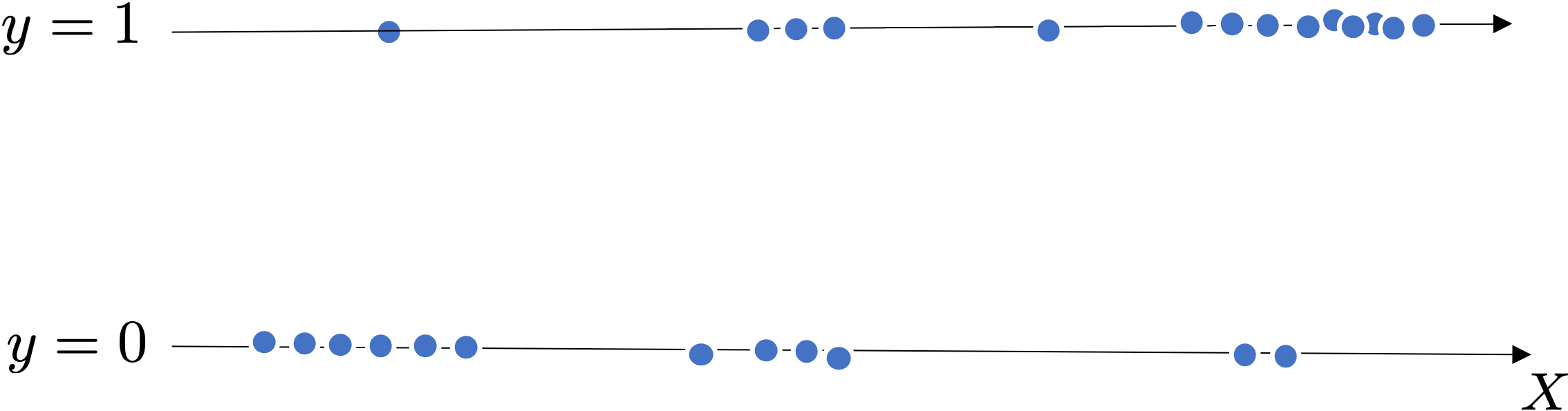
y = (X > 0).astype(float)
X[X > 0] *= 4
X += 0.3 * np.random.normal(size=n_samples)
X = X[:, np.newaxis]
plt.plot(X[y==1],[0]*sum(y==1),'.')
plt.plot(X[y==0],[0]*sum(y==0),'r.');

import numpy as np
import matplotlib.pyplot as plt

from sklearn.linear_model import LogisticRegression, LinearRegression
from scipy.special import expit


# Fit the classifier
clf = LogisticRegression(C=1e5)
clf.fit(X, y)

# and plot the result
plt.figure(1, figsize=(8, 6))
plt.clf()
plt.scatter(X.ravel(), y, color="black", zorder=20)
X_test = np.linspace(-5, 10, 300)

loss = expit(X_test * clf.coef_ + clf.intercept_).ravel()
plt.plot(X_test, loss, color="red", linewidth=3)

ols = LinearRegression()
ols.fit(X, y)
plt.plot(X_test, ols.coef_ * X_test + ols.intercept_, linewidth=1)
plt.axhline(0.5, color=".5")

plt.ylabel("y")
plt.xlabel("X")
plt.xticks(range(-5, 10))
plt.yticks([0, 0.5, 1])
plt.ylim(-0.25, 1.25)
plt.xlim(-4, 10)
plt.legend(
    ("data","Logistic Regression Model", "Linear Regression Model"),
    loc="lower right",
    fontsize="small",
)
plt.tight_layout()
plt.show()

from sklearn.datasets import make_classification

X, y = make_classification(
    n_features=2, n_redundant=0, n_informative=2, n_clusters_per_class=1, random_state=0, class_sep=0.8)
plt.scatter(*X.T,c=y,cmap=cm.get_cmap("RdBu"));

clf = LogisticRegression(penalty='none')
clf.fit(X, y); minx, maxx = X.min(), X.max()
support = np.linspace(minx, maxx, 100)
xx, yy = np.meshgrid(support, support)
points = np.stack((xx.flatten(), yy.flatten()), axis=1)
prob_mesh = clf.predict_proba(points)
prob_mesh = prob_mesh[:,0].reshape(xx.shape)
fig, axes = plt.subplots(1,2,figsize=(12,6))
axes[0].contourf(xx,yy,prob_mesh,cmap=cm.get_cmap("RdBu"));axes[0].plot(0,0,'rx')
axes[0].scatter(*X.T,c=(1-y),cmap=cm.get_cmap("RdBu"));
axes[0].axis('scaled');axes[1].bar([0,1],clf.coef_[0]);axes[1].axis('equal');axes[1].set_xlim((-5,5));axes[1].set_ylim((-2,8));

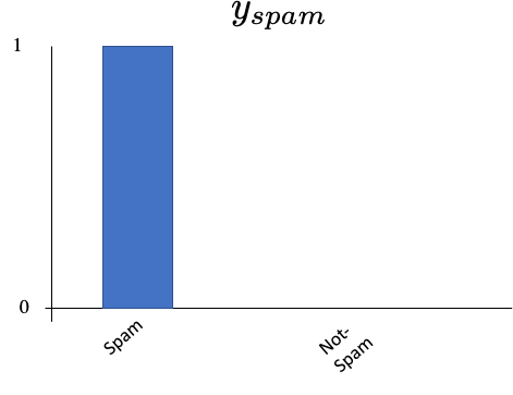
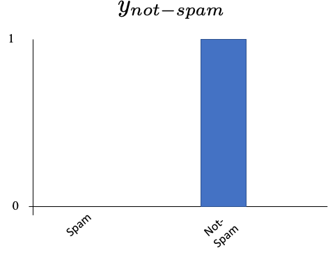
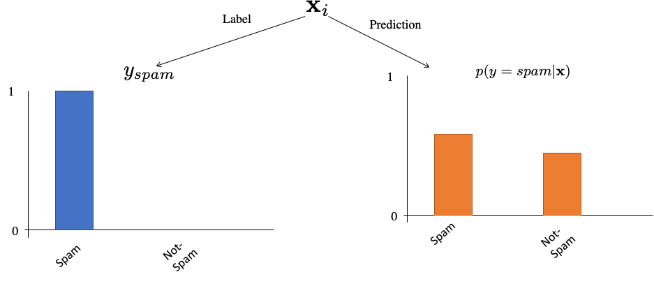
[1,0] and [0,1] are possible for 2 classes since it has to be a prob. distribution[1,1] is not a prob. distributionSo for a $K=2$ binary class problem,e.g. (spam vs not-spam) the possible labels could be:
$$ y_{spam} = [1, 0]^T$$$$ y_{not-spam} = [0, 1]^T$$
Who can tell me how we can compare two [discrete] probability distributions?
Objective: Estimate a sort of "distance" (or better divergence) between two distributions $p(x)$ vs $q(x)$.
If we use $q(x)$ to construct a coding scheme for the purpose of transmitting values of $x$ to a receiver instead of $p(x)$, then the average additional amount of information required to specify the value of $x$ as a result of using $q(x)$ instead of the true distribution $p(x)$ is given by:
$$ \underbrace{H(P,Q)}_{\text{q not p, so extra}} - \underbrace{~~H(P)~~}_{\text{best we can do}} $$Idea: if you use q instead of p, but the underlying process is governed by p, then you need to pay an extra price in transmission a bit more of information. "The bit more" is the equation above.
We can use KL divergence!
$$ KL(P||Q) = H(P,Q) - H(P) = \underbrace{-\sum_{x \in X} p(x)\log q(x)}_{\text{cross-entropy}} - \underbrace{\big(-\sum_{x \in X} p(x)\log p(x)\big)}_{\text{entropy}} $$Note that:
Wait a second but....how much is the entropy of the "labels" aka entropy of $[0,1]$ or $[1,0]$?
$$
H(P,Q) - H(P) = \underbrace{-\sum_{x \in X} p(x)\log q(x)}_{\text{cross-entropy}} - \underbrace{\big(-\sum_{x \in X} p(x)\log p(x)\big)}_{\text{entropy of labels is zero}}
$$
Maximizing Log Likelihood - I removed the sum over training samples for clarity
$$ \begin{aligned} &\log L(\theta)= y^{(i)}\log p\left(x^{(i)}\right)+\left(1-y^{(i)}\right) \log \left(1-p\left(x^{(i)}\right)\right) \end{aligned} $$Minimizing Cross-Entropy
$$ \begin{aligned} H(P,Q) - H(P) = \underbrace{-\sum_{y \in Y} p(y|x)\log q(y|x)}_{\text{cross-entropy}} \\ -\Big(p(y=1)\log q(y=1|x)+p(y=0)\log q(y=0|x)\Big)\\ -\Big(p(y=1)\log q(y=1|x)+(1-p(y=1))\log (1-q(y=1|x))\Big)\\ -\Big(y\log q(y=1|x)+(1-y)\log (1-q(y=1|x))\Big)\\ \end{aligned} $$Maximizing Log Likelihood
$$y \log p\left(x\right)+\left(1-y\right) \log \left(1-p\left(x\right)\right) $$Minimizing Cross-Entropy $$-\Big(y\log q(y=1|x)+(1-y)\log (1-q(y=1|x))\Big)$$

1 in the label.multiple choice questionsThe questions will be of increasing difficulties and calibrated to the test time.
Given the following training data for a $\{0, 1\}$ binary classifier
Determine the output of a K Nearest Neighbour (K-NN) classifier for all points on the interval $0 \le x \le 1$ using:
Will be majority vote of class labels since we classify using all training points. Aka, we have two "1" and one "0". So always 1!
A regressor algorithm is defined using the mean of the K Nearest Neighbours of a test point. Determine the ouput on the interval $0 \le x \le 1$ using the training data in the previous example for $K=2$.
So we want to reduce 1) Misclassification or 2)Gini Impurity or 3) ? What else ?
Know your enemy: the uniform distributions $\mbf{x} \sim\mathcal{U}$
We want find a function $f(p)$ so that $f(p)$ is very distant from uniform distribution $Q$, so we can use KL divergence for this:
$$ KL(P||Q)= \sum_{k=1}^K p(x)\log \Big( \frac{p(x)}{1/K} \Big) = \sum_{k=1}^K p(x)\log\big(p(x)\big)-p(x)\log\big(1/K\big) $$You and your best friend found a trick to save bandwidth over the internet. Instead of sharing a total of $N=10M$ grayscale images directly over the Internet, you took the $N$ images and learned $K=1000$ centroids $\{\mu_1,\ldots,\mu_{K}\}$ using K-means. Each input image is defined over the set $\mbf{x} \in [0,255]^{H\times W \times 1}$. Then you shared once for all the $K$ centroids $\{\mu_k\}_{k=1}^{K}$ with your friend.
Easy Questions: (check if you know the basic notions)
More Difficult Questions: (check if you can reason on problems)
You send $y$ associated to the image $\mbf{x}$, so $y$ takes value in $[1,K]$ and you friend can use $y$ to select the centroid nearest to the point $\mbf{x}$.
In fact, the point $\mbf{x}$ was clustered in the cluster given by $y$.
So one could stop here and say that the best approximation for $\mbf{x}$ is $\mu_{y}$ ($\mbf{x} \approx \mu_{y}$) but we can do more.
Given that we have the scalar euclidean distance between $\mbf{x}$ and the associated centroid aka $\mu_{y}$ we have:
$$ d= \vert \vert \mbf{x} -\mu_{y} \vert \vert_2$$We have only $d$ and $\mu_{y}$, the image $\mbf{x}$ that was sent is in the set:
$$ \{\forall~\mbf{v} \in [0,255]^{H\times W \times 1}: \vert \vert \mbf{v} - \mu_y \vert \vert_2 = d \}$$which is all the points in the hyper-sphere in $[0,255]^{H\times W \times 1}$ of radius $d$ and centered at $\mu_y$
You are hired by a famous company that has to compute $\ell_2^2$ norm over two feature vectors $\mbf{x} \in \mathbb{R}^{D}$ and $\mbf{y}\in \mathbb{R}^{D}$.
The company works with a machine learning algorithm that guarantees that the features $\mbf{x}$ and $\mbf{y}$ lie on a unit hyper-sphere (_Hint: same as $\vert \vert x \vert\vert_2^2 =1$)_
$$ d^2 = \vert \vert \mbf{x} - \mbf{y} \vert\vert_2^2 = \sum_{i=1}^D (x_i - y_i)^2$$(Hint: develop the definition of the norm written above)
Using unit hyper-sphere: $$1 + 1 - 2 \mbf{x}^T\mbf{y} = 2 - 2 \mbf{x}^T\mbf{y}$$
So, yes, they can simply computing the dot product multiply by -2 and add 2.
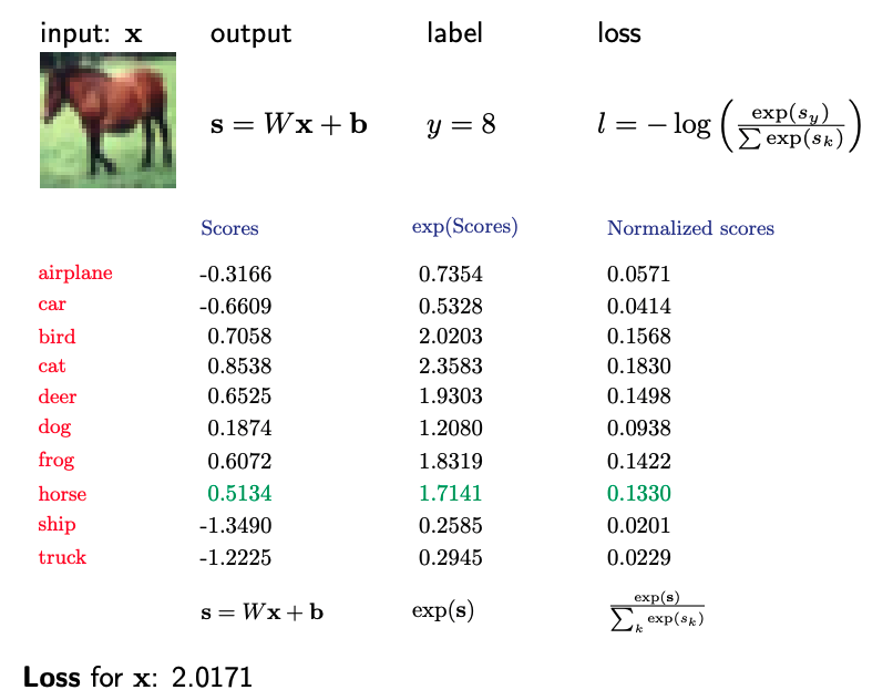
| Data Type $y$ | Expo. Family | Name |
|---|---|---|
| $\{1,K\}$ | Categorical | Multi-class Classification |

$\mbf{x}$ is assigned to point with higher distance to the hyper-plane (because it is more confident to be that class).

$\mbf{x}$ is assigned to point with lower distance to the hyper-plane (because it the least unsure).

$\mbf{x}$ is assigned to point with lower distance to the hyper-plane (because it the least unsure).

import numpy as np
ww = [[1, 2], [-1, 4], [8, 2]]
support = np.linspace(-10, 10, 100)
xx, yy = np.meshgrid(support, support)
W = np.array(ww)
dim = xx.shape
points = np.stack((xx.flatten(), yy.flatten()), axis=1)
dist = np.argmax((W@points.T), axis=0)
dist = dist.reshape(dim)
plt.figure(figsize=(7,7))
plt.contourf(xx, yy, dist, cmap='jet')
plt.plot(0, 0, 'rx')
plt.axis('scaled')
#plt.colorbar()
plt.xlim(-10, 10);

Binary case: $$ \operatorname{sign}\big(\mbf{w}^T\mbf{x}_i + b\big) > 0 $$
$$\operatorname{sign}(z)= \begin{cases} +1, & \mbox{if } z\ge0 \\ -1, & \mbox{if } z<0\end{cases}$$let's consider the distance as:
We want:
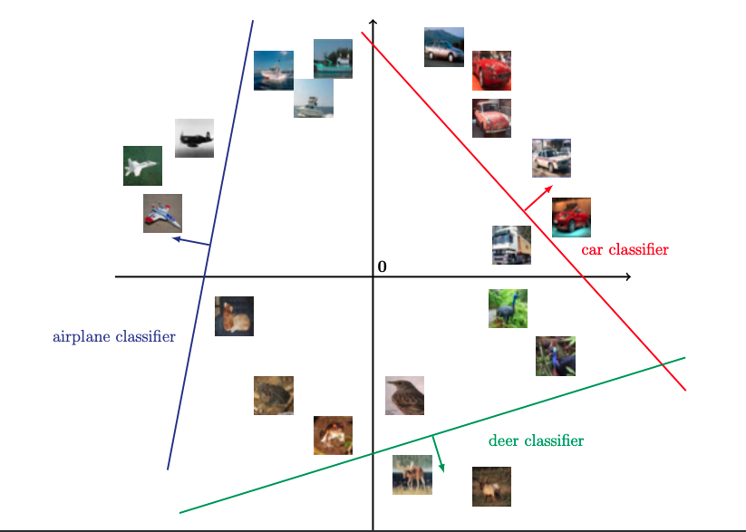
$$ \begin{cases} \mbf{w}^T\mbf{x} + b > 0 \quad y=+1\\ \mbf{w}^T\mbf{x} + b < 0 \quad y=-1\\ \end{cases} $$Decision boundary $\{\mbf{w}_k,b_k\}_{k=1}^K$ per class given K classes.
$$ \begin{align} f_{\{\mbf{w}_1,b_1\}} = \mbf{w}_1^T\mbf{x} + b_1 \quad y=1\\ f_{\{\mbf{w}_2,b_2\}} = \mbf{w}_2^T\mbf{x} + b_2 \quad y=2\\ \cdots \\ f_{\{\mbf{w}_K,b_K\}} = \mbf{w}_K^T\mbf{x} + b_K \quad y=K\\ \end{align} $$Decision boundary $\{\mbf{w}_k,b_k\}_{k=1}^K$ per class given K classes.
A data point $\mbf{x}^{\star}$ is assigned to class $\hat{k}$ iff:
$$f_{\{\mbf{w}_\hat{k},b_\hat{k}\}}\big(\mbf{x}^{\star}\big) > f_{\{\mbf{w}_j,b_j\}}\big(\mbf{x}^{\star}\big) \quad \forall j \in \{1,\ldots K\} \setminus\{\hat{k}\} $$let's write it explicitly
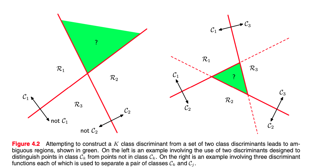
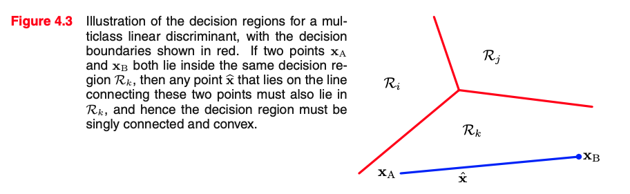
This has the same form as the decision boundary for the two-class case discussed before.
The decision regions of such a discriminant are always singly connected and convex.
Assuming $\mbf{x}_A$ and $\mbf{x}_B$ are in $\mathcal{R}_k$:
$$ \begin{align} (\mbf{w}_{k}-\mbf{w}_{j})^T{\mbf{x}_A} + (b_{k}- b_{j}) > 0 \quad \forall j\neq k\\ (\mbf{w}_{k}-\mbf{w}_{j})^T{\mbf{x}_B} + (b_{k}- b_{j}) > 0 \quad \forall j\neq k\\ \end{align} $$and also (definition of convexity): $$ \hat{\mbf{x}} = \lambda\mbf{x}_A + (1-\lambda)\mbf{x}_B ~~~\text{with}~~~~ 0 \le \lambda \le 1$$
Then also $\hat{\mbf{x}}$ is in $\mathcal{R}_k$, where $f_k(\cdot)$ is the hyper-plane: $$ f_k(\hat{\mbf{x}}) > f_j(\hat{\mbf{x}})\quad \forall j\neq k$$
We have to show that: $$ f_k(\hat{\mbf{x}}) > f_j(\hat{\mbf{x}})\quad \forall j\neq k$$
and we know that $f_k({\mbf{x}}_A) > f_j({\mbf{x}}_A)$ and $f_k({\mbf{x}_B})>f_j({\mbf{x}_B}) ~~\forall j\neq k$ holds.
We apply the definition and use linearity of hyper-plane (dot product):
$$ \hat{\mbf{x}} = \lambda\mbf{x}_A + (1-\lambda)\mbf{x}_B ~~~\text{with}~~~~ 0 \le \lambda \le 1$$$$f_k(\hat{\mbf{x}})= f_k\Big( \lambda\mbf{x}_A + (1-\lambda)\mbf{x}_B\Big) = \lambda f_k( \mbf{x}_A) + (1-\lambda)f_k( \mbf{x}_B)$$Same hold for: $$f_j(\hat{\mbf{x}})= f_k\Big( \lambda\mbf{x}_A + (1-\lambda)\mbf{x}_B\Big) = \lambda f_j( \mbf{x}_A) + (1-\lambda)f_j( \mbf{x}_B)$$
Now this holds by assumption $$ f_k({\mbf{x}}_A) > f_j({\mbf{x}}_A) \quad \forall j\neq k$$ given that $f_k({\mbf{x}_B})>f_j({\mbf{x}_B})$, it must be:
$$ f_k({\mbf{x}}_A) + f_k({\mbf{x}_B}) > f_j({\mbf{x}}_A) + f_j({\mbf{x}_B}) \quad \forall j\neq k$$We have to prove: $$f_k(\hat{\mbf{x}})= f_k\Big( \lambda\mbf{x}_A + (1-\lambda)\mbf{x}_B\Big) = \lambda f_k( \lambda\mbf{x}_A) + (1-\lambda)f_k( \lambda\mbf{x}_B)$$ We arrived here: $$ f_k({\mbf{x}}_A) + f_k({\mbf{x}_B}) > f_j({\mbf{x}}_A) + f_j({\mbf{x}_B}) \quad \forall j\neq k$$
Remember $0 \le \lambda \le 1$ thus both $\lambda \ge 0$ and $(1-\lambda) \ge 0$, thus:
$$ \underbrace{\lambda f_k({\mbf{x}}_A) + (1-\lambda)f_k({\mbf{x}_B})}_{f_k(\hat{\mbf{x}})} > \underbrace{\lambda f_j({\mbf{x}}_A) + (1-\lambda)f_j({\mbf{x}_B})}_{f_j(\hat{\mbf{x}})} \quad \forall j\neq k$$
Thus convex linear combination $\hat{\mbf{x}}$ still satisfy the same decision boundary:
$$f_k(\hat{\mbf{x}}) > f_j(\hat{\mbf{x}}) \quad \forall j\neq k$$Decision boundary $\{\mbf{w}_k,b_k\}_{k=1}^K$ per class given K classes.
$$ \begin{align} f_{\{\mbf{w}_1,b_1\}} = \mbf{w}_1^T\mbf{x} + b_1 \quad y=1\\ f_{\{\mbf{w}_2,b_2\}} = \mbf{w}_2^T\mbf{x} + b_2 \quad y=2\\ \cdots \\ f_{\{\mbf{w}_K,b_K\}} = \mbf{w}_K^T\mbf{x} + b_K \quad y=K\\ \end{align} $$Decision boundary $\{\mbf{w}_k,b_k\}_{k=1}^K$ per class given K classes.
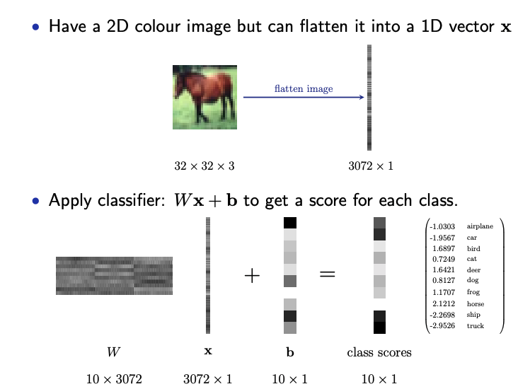
We can model directly everything with a matrix:
$$ \underbrace{\mbf{y}}_{\mathbb{R}^{Kx1}} = \underbrace{\mbf{W}}_{\mathbb{R}^{K\times d}}\underbrace{\mbf{x}}_{\mathbb{R}^{d\times1}} + \underbrace{\mbf{b}}_{\mathbb{R}^K}$$Will this work?
$$ \underbrace{\mbf{Y}}_{\mathbb{R}^{Kxn}} = \underbrace{\mbf{W}}_{\mathbb{R}^{K\times d}}\underbrace{\mbf{X}}_{\mathbb{R}^{d\times n}} + \underbrace{\mbf{b}}_{\mathbb{R}^K}$$OK there is broadcasting on $\mbf{b}$!
Can I just do
y = np.argmax(W@points.T, axis=0)
if I want to train a model?
$$\arg\max_{\mbf{W},\mbf{b}}\Big[\arg\max_k \big(\mbf{W}\mbf{X} + \mbf{b} \big)\Big]$$argmax itself differentiable?¶import numpy as np
from scipy.special import softmax
_softmax = False
ww = [[1, 2], [-1, 4], [8, 2]];support = np.linspace(-10, 10, 100)
xx, yy = np.meshgrid(support, support)
W = np.array(ww)
dim = xx.shape
points = np.stack((xx.flatten(), yy.flatten()), axis=1)
prob = np.argmax(W@points.T, axis=0) if not _softmax else np.max(np.tile(
np.arange(0, 3).T, (points.shape[0], 1)).T*softmax(0.2*W@points.T, axis=0), axis=0)
prob = prob.reshape(dim)
plt.figure(figsize=(7, 7));
plt.contourf(xx, yy, prob, cmap='jet');plt.plot(0, 0, 'rx');plt.axis('scaled');plt.xlim(-10, 10);plt.figure(figsize=(7, 7));
ax = plt.axes(projection='3d');ax.plot_surface(xx, yy, prob,rstride=1, cstride=1,cmap='jet', edgecolor='none');ax.view_init(30, -110)

argmax with a smooth differentiable version called SoftMax is rather a smooth approximation to the arg max function: the function whose value is which index has the maximum, modeled as One-Hot Encoding
Think Softmax as a differentiable selector!
import numpy as np
from scipy.special import softmax
_softmax = True
ww = [[1, 2], [-1, 4], [8, 2]]
support = np.linspace(-10, 10, 100)
xx, yy = np.meshgrid(support, support)
W = np.array(ww)
dim = xx.shape
points = np.stack((xx.flatten(), yy.flatten()), axis=1)
prob = np.argmax(W@points.T, axis=0) if not _softmax else np.max(np.tile(
    np.arange(0, 3).T, (points.shape[0], 1)).T*softmax(0.2*W@points.T, axis=0), axis=0)
prob = prob.reshape(dim)
plt.figure(figsize=(7, 7))
plt.contourf(xx, yy, prob, cmap='jet')
plt.plot(0, 0, 'rx')
plt.axis('scaled')
# plt.colorbar()
plt.xlim(-10, 10);
plt.figure(figsize=(7, 7))
ax = plt.axes(projection='3d')
ax.plot_surface(xx, yy, prob,rstride=1, cstride=1,
                cmap='jet', edgecolor='none')
ax.view_init(30, -130)


argmax¶import numpy as np
from scipy.special import softmax
_softmax = True
temperature = 10
ww = [[1, 2], [-1, 4], [8, 2]]
support = np.linspace(-10, 10, 100)
xx, yy = np.meshgrid(support, support)
W = np.array(ww)
dim = xx.shape
points = np.stack((xx.flatten(), yy.flatten()), axis=1)
prob = np.argmax(points, axis=1) if not _softmax else np.max(np.tile(
np.arange(0, 2).T, (points.shape[0], 1))*softmax(temperature*points, axis=1), axis=1)
prob = prob.reshape(dim)
plt.figure(figsize=(4, 4))
plt.contourf(xx, yy, prob, cmap='jet', levels=500)
plt.plot(0, 0, 'rx');plt.axis('scaled');plt.xlim(-10, 10);plt.figure(figsize=(7, 7));ax = plt.axes(projection='3d')
ax.plot_surface(xx, yy, prob,rstride=1, cstride=1,
cmap='jet', edgecolor='none')
ax.view_init(30, 30)


We model conditional probability of $y|x$:
$$ \begin{cases} p(y=1| \mbf{x};\mbf{W},\mbf{b}) = p_1 = \bmf{\sigma}_1\left( \mbf{W}\mbf{X} + \mbf{b} \right)\\ p(y=2| \mbf{x};\mbf{W},\mbf{b}) = p_2 = \bmf{\sigma}_2\left( \mbf{W}\mbf{X} + \mbf{b} \right)\\ \ldots \\ p(y=K| \mbf{x};\mbf{W},\mbf{b}) = p_K = \bmf{\sigma}_K\left( \mbf{W}\mbf{X} + \mbf{b} \right)\\ \end{cases} $$
$$f_{\boldsymbol{\theta}}(\mbf{x}) \doteq \bmf{\sigma}\left( \mbf{W}\mbf{X} + \mbf{b} \right)$$
where:
$$ \bmf{\sigma}_i(z)= \frac{e^{z_i}}{\sum_{k=1}^K e^{z_k}} \quad \text{Softmax function}$$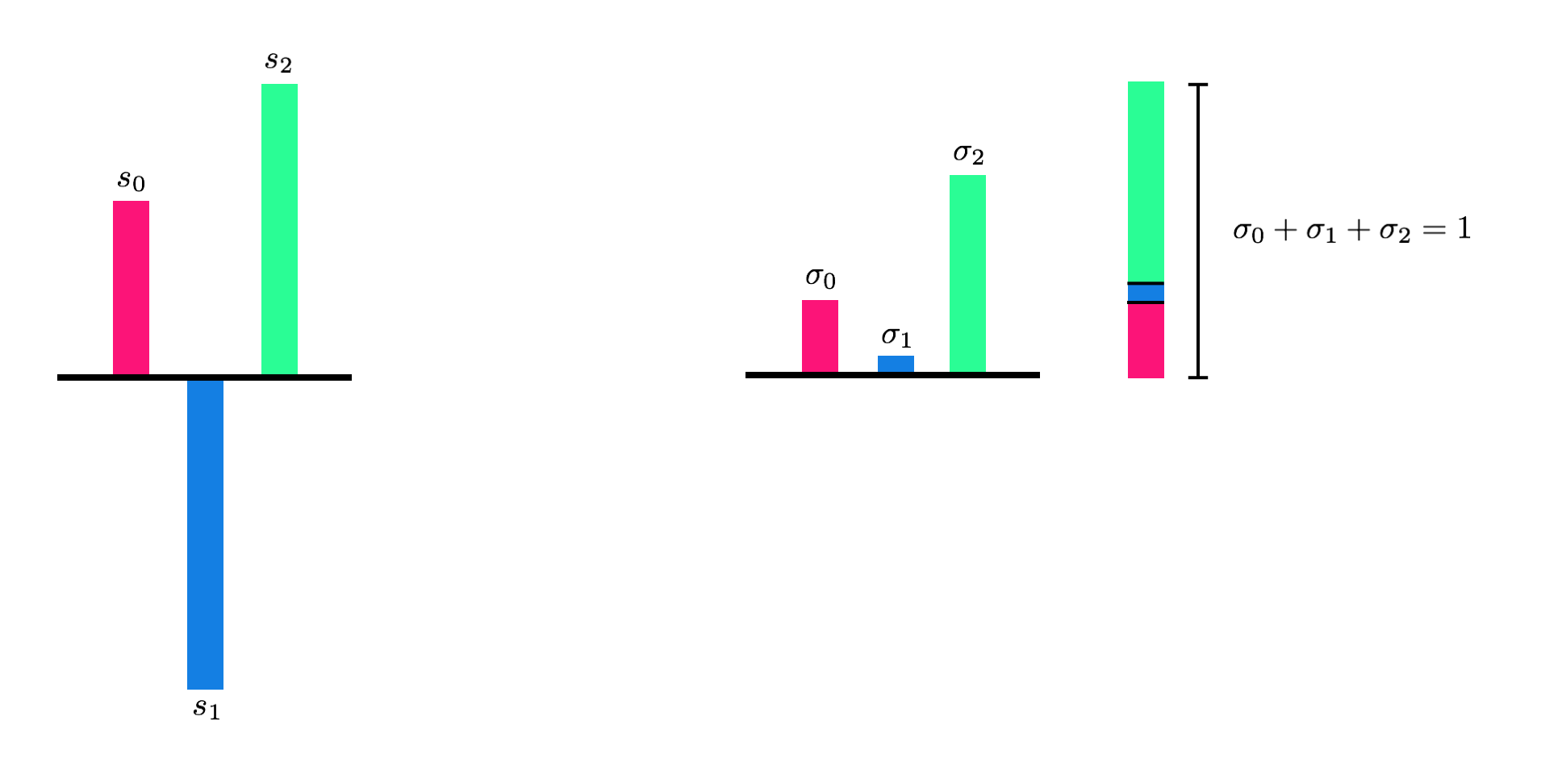
you can think $\mbf{z} = \mbf{W}\mbf{x}+\mbf{b}$ as unormalized log-probability of each class.
$$ p(\mbf{y}| \mbf{x};\mbf{W},\mbf{b}) = \frac{\exp({\mbf{W}_y\mbf{x}+\mbf{b})}}{\sum_{k=1}^K\exp({\mbf{W}_k\mbf{x}+\mbf{b}_k)}} $$you can think $\mbf{z} = \mbf{W}\mbf{x}+\mbf{b}$ as unormalized log-probability of each class.
$$ p(\mbf{y}| \mbf{x};\mbf{W},\mbf{b}) = \frac{\exp({\mbf{W}\mbf{x}+\mbf{b})}}{\sum_{k=1}^K\exp({\mbf{W}_k\mbf{x}+\mbf{b}_k)}} $$unormalized log-probability

NameError: name 'softmax' is not defined

Let's say that you have a model and you sample the weights $\mbf{W},\mbf{b}$ randomly from some distributions so that they are non zero. Also assume that the data $\mbf{x}$ is meaningful (non-zero).
Can get you
nanas $+\infty$ in the loss while you start training? Or better, which is the value of the loss as soon as you start training?
nan as $+\infty$.
Yes, almost the same (up to save/wasted space)
$$ p(\mbf{y}| \mbf{x};\mbf{W},\mbf{b}) = \frac{\exp({\mbf{W}\mbf{x}+\mbf{b})}}{\sum_{k=1}^K\exp({\mbf{W}_k\mbf{x}+\mbf{b}_k)}} $$Now $K=2$ and define $\mbf{z} \doteq \mbf{W}\mbf{x} + \mbf{b}$:
$$ p(\mbf{y}=1| \mbf{x};\mbf{W},\mbf{b}) = \frac{\exp(\mbf{z}_1)}{\sum_{k=1}^K\exp(\mbf{z}_k)} = \frac{\exp(\mbf{z}_1)}{\exp(\mbf{z}_1) + \exp(\mbf{z}_2)} $$Yes it is the same but with sigmoid you spare a vector since $\mbf{W}$ becomes a single vector $\mbf{w}$ not a matrix!
We can avoid modeling the other class since $ p(\mbf{y}=0| \mbf{x};\mbf{W},\mbf{b})=1- p(\mbf{y}=1| \mbf{x};\mbf{W},\mbf{b})$