Machine Learning

AI & Machine Learning - Unit 2

---

5. Clustering with K-means

Prof. Iacopo Masi - Computer Science Department, Sapienza University of Rome

Recap previous lecture

• Principal Components Analysis (PCA)
• Eigendecomposition of a matrix
• Geometry behind PCA
• Application of PCA for:
  • Compressing the data (point cloud to line)
  • Modeling 3D Faces (3D Morphable Model 3DMM)
  • Rotating the data

Today's lecture

Unsupervised Learning: Clustering

K-means

Coordinate Descent

Application: Pixel Segmentation

Image recognition: Visual Bag of Words (hints)

This lecture material is taken from

• Cimi Book - Chapter 15
• Bishop - Chapter 9.1
• Stanford Kmeans
• Stanford Kmeans
• Illustrations
• Code

Unsupervised Learning

Objective and Motivation: The goal of unsupervised learning is to find hidden patterns in unlabeled data.

\begin{equation} \underbrace{\{\mathbf{x}_i\}_{i=1}^N}_{\text{known}} \sim \underbrace{\mathcal{D}}_{\text{unknown}} \end{equation}

• Unlike in supervised learning, any data point is not paired with a label.

• As you can see the unsupervised learning problem is ill-posed (which hidden patterns?) and in principle more difficult than supervised learning.

• Unsupervised learning can be thought of as "finding structure" in the data.

Unsupervised Learning

• PCA and matrix factorization methods such as Eigendecomposition and Singular Value Decomposition (SVD)
• "Hidden Patterns" and "Finding Structure" translate into finding a low-dimensional embedding of the data.
• Usage:
  • Visualization of high-dimensional data
  • Dimensionality Reduction
  • Compression and Noise Filtering
  • Further pre-processing by machine learning algorithms
  • Decorrelate the features (i.e. covariance matrix is diagonal)

Unsupervised Learning: Clustering

• "Hidden Patterns" and "Finding Structure" translate into deriving a partitioning of the data into clusters.

plt.scatter(X[:, 0], X[:, 1], c='black', marker='o', s=50)
plt.show()

plt.scatter(X[:, 0], X[:, 1], c=y, marker='o', s=50, cmap='jet')
plt.show()

Supervised Learning is more constrained

• The mapping data to color (labels) is given
• With clustering, we are given just a point cloud of data with no label assigned

Clustering is ill-posed

from sklearn.datasets import make_blobs

X2, y2 = make_blobs(n_samples=150, 
                  n_features=2, 
                  centers=3, 
                  cluster_std=.7, 
                  shuffle=True, 
                  random_state=0)

plt.scatter(X2[:, 0], X2[:, 1], c='black', marker='o', s=50)
plt.show()

• How many clusters are here, three or two?

Why Clustering is useful

• Applications:
  • Color Compression
  • Vector "quantization"
  • Data compression
  • Image Retrieval (codebook) --> Bag of Visual Words
  • Finding "groups" given points in a vector space
    • I.e. Marketing Department: you have a customer as a vector.
      • Each axis of the vector indicates 1) annual income 2) Age 3) Location etc.
      • Objective: Identify "groups" of customers to have an ad-hoc advertising campaign.

Clustering: formalizing the problem

• Input:
  1. $\quad$ A set of points $\{ \mbf{x}_1, \ldots, \mbf{x_n}\}$ in a d-dim vector space $\mbf{x} \in \mathbb{R}^d$,
  2. $\quad$ $k$ number of clusters to find

• Output:
  1. $\quad$ A set of points "centroids" $\{ \mbf{\mu}_1, \ldots, \mbf{\mu}_k\}$ where $\mbf{\mu} \in \mathbb{R}^d$,
  2. $\quad$ A list of assignment labels that create a mapping from data points to centroids $\{ y_1, \ldots, y_n\}$
  3. $\quad$ The clusters are meant to be disjoint (there is no overlap between clusters).

• Note that $y$ is a scalar $\in [1,\ldots,k]$
• The assignment labels map a data point to a single centroid
• It conveys the information: data points 3 maps to the cluster centroid 2
• For this to work formally the $y_i$ needs to be aligned with $\mbf{x}_i$

plt.scatter(X[:, 0], X[:, 1], c='black', marker='o', s=50)
plt.show()

from sklearn.cluster import KMeans

km = KMeans(n_clusters=3, 
            init='random', 
            n_init=10, 
            max_iter=300,
            tol=1e-04,
            random_state=0)
y_km = km.fit_predict(X)

plt.scatter(X[y_km == 0, 0],
            X[y_km == 0, 1],
            s=50,
            c='lightgreen',
            marker='s',
            label='cluster 1')
plt.scatter(X[y_km == 1, 0],
            X[y_km == 1, 1],
            s=50,
            c='orange',
            marker='o',
            label='cluster 2')
plt.scatter(X[y_km == 2, 0],
            X[y_km == 2, 1],
            s=50,
            c='lightblue',
            marker='v',
            label='cluster 3')
plt.scatter(km.cluster_centers_[:, 0],
            km.cluster_centers_[:, 1],
            s=250,
            marker='*',
            c='red',
            label='centroids')
plt.legend()
plt.tight_layout()
plt.show()

Clustering: K-means Algorithm

• Solving this problem in an optimal way is an NP-Hard problem
• A non-optimal solution to this problem can be obtained with the K-means algorithm.
• In practice, K-means plus other heuristics make the approach usable in multiple problems.

Remember that we have to find:

1. $\quad$ A set of points "centroids" $\{ \mbf{\mu}_1, \ldots, \mbf{\mu}_k\}$ where $\mbf{\mu} \in \mathbb{R}^d$,
2. $\quad$ A list of assignment labels that create a mapping from data points to centroids $\{ y_1, \ldots, y_n\}$

Let's think how we can solve it

What would you do?

plt.scatter(X[:, 0], X[:, 1], c='black', marker='o', s=50)
plt.show()

1. We need some "reference" centroids to start

• Initialization: Random sample the $K$ centroids $\{ \mbf{\mu}_1, \ldots, \mbf{\mu}_k\}$

• A trick is using available points (just choose a few of them)

  

  Figures Credit

2. Assignment Step

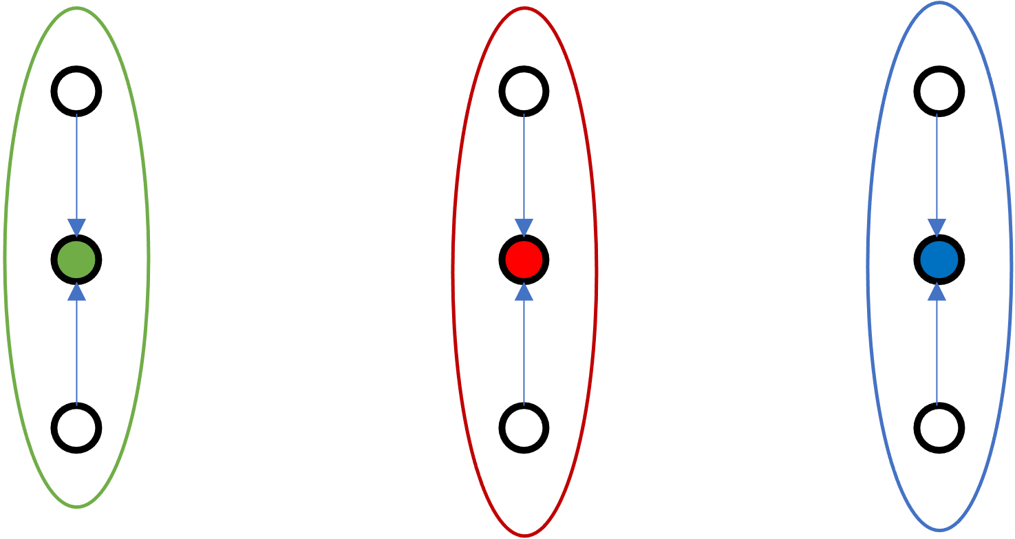
• For every point $i=[1,\ldots,N]$ compute the assignment wrt to the $K$ clusters.

  • We have to compare $N\times K$ points (#data points x #clusters)

  • Given a point $\mbf{x}_i$, we have to find the label of the "closest" centroids in $\{ \mbf{\mu}_1, \ldots, \mbf{\mu}_k\}$

    • $y_i = \arg\min_k || \mbf{x}_i -\mbf{\mu}_k ||_2^2 $

    

• At the end of this step we should have a pair of aligned set $\{ \mbf{x}_1, \ldots, \mbf{x_n}\}$ and $\{ {y}_1, \ldots, {y_n}\}$

3. Update Step

• Now, it is the inverse of before. Now we consider the "centroids".
• For every centroid $k=[1,\ldots,K]$ we update its mean based on the previous assignments:

• Given a $\mbf{\mu}_k$, we update it as $\mbf{\mu}_k \leftarrow \frac{\sum_i \delta\{y_i=k\}\mbf{x}_i}{\sum_i \delta\{y_i=k\}}$

  

• At the end of this step we should have a pair of aligned set $\{ \mbf{x}_1, \ldots, \mbf{x_n}\}$ and $\{ {y}_1, \ldots, {y_n}\}$ and updated centroids $\{ \mbf{\mu}_1, \ldots, \mbf{\mu}_k\}$.

Indicator function

$$ \delta_{ij} = \begin{cases} 0 &\text{if } i \neq j, \\ 1 &\text{if } i=j. \end{cases} $$

It is a formalism to express the concept of:

• DO consider the point in the mean computation if point label corresponds to current centroid
• DO NOT consider the point in the mean computation if the point label DOES NOT correspond to the current centroid

Final result

K-means (Lloyd’s method)

1. Random init of centroids
2. Repeat until convergence:
   • Assignment step: $\forall i\in[1,N] \quad y_i = \arg\min_k || \mbf{x}_i -\mbf{\mu}_k ||_2^2 $
   • Update step: $\forall k\in[1,K] \quad \mbf{\mu}_k \leftarrow \frac{\sum_i \delta\{y_i=k\}\mbf{x}_i}{\sum_i \delta\{y_i=k\}}$

What does "convergence" mean?

K-means convergence

• One could check that the centroids do not change anymore (up to some $\epsilon$), even performing more steps.
• Is there a better "convergence" term? (we will look into this later)

Let's implement a basic version with numpy

We start from this 150 points in 2-D space

print(X.shape[0])
print(X.shape[1])

150
2

plt.scatter(X[:, 0], X[:, 1], c='black', marker='o', s=50); 
plt.show()

def init(X, k):
    N, dim = X.shape
    # we select k samples from the points we have randomly
    idx = np.random.choice(N, k, replace=False)
    # the centers are just the k-random sampled points
    return X[idx]


def get_assignments(X, centers):
    P = X[:, np.newaxis, :]  # Nx1xD
    diff_sq = (P - centers)**2  # Nx1xD - KxD -> NxKxD # broadcasting
    # more info on broadcasting https://numpy.org/doc/stable/user/basics.broadcasting.html
    # dist = sum_over_axis(diff^2) then take argmin of dist across centers
    y = diff_sq.sum(axis=2).argmin(axis=1)
    return y  # Nx1 and the values inside go from [1...K]


def update_centers(X, y, K):
    # select the points to the k center and remove the N dimension with mean over axis 0
    y_row = y.reshape((1, -1)) #1xN
    k_col = np.arange(K).reshape(-1, 1) #Kx1
    
    #M[i][j] = 1 if X[j,:] belongs to cluster i else 0 
    M = k_col == y_row  #KxN
    
    #cluster_sum[i,:] contains the sum of all vectors in cluster i
    cluster_sum = M @ X #KxN @ NxD -> KxD 
    
    #counts[i,:] contains the number of vectors in cluster i
    counts = np.sum(M, axis=1).reshape(-1, 1) #Kx1
    
    return cluster_sum / counts #KxD

# Double check
np.random.seed(0)  # make the method deterministic
from sklearn.metrics import pairwise_distances_argmin
centers = init(X, 3)
y_assignments = get_assignments(X, centers)
labels = pairwise_distances_argmin(X, centers)
assert np.array_equal(labels, y_assignments), 'Assignment not correct!'

def kmeans(X, n_clusters):
    np.random.seed(0)  # make the method deterministic
    iter = 1
    #1. init random sample the centers
    centers = init(X, n_clusters)
    
    while True:
        # 2. Assignment step 
        y_assignments = get_assignments(X, centers)
        
        # 3. Update step
        new_centers = update_centers(X, y_assignments, n_clusters)
        
        # 4. Check for convergence
        # This is a possible implementation
        # A more formal is to check that the loss is plateauing (more on this later)
        if np.allclose(centers, new_centers):
            break
        # update cluster for next iter
        centers = new_centers
        
        print(f'Iteration {iter}')
        iter += 1
    
    return centers, y_assignments

centers, y_est = kmeans(X, 3)
plt.scatter(*X.T, c=y_est,
            s=50, cmap='viridis')
_ = plt.scatter(*centers.T,
                s=250,
                marker='*',
                c='red',
                label='centroids')

Iteration 1
Iteration 2
Iteration 3

Let's try a larger dataset

from sklearn.datasets import make_blobs

X, y = make_blobs(n_samples=5000, 
                  n_features=3, 
                  centers=25, 
                  cluster_std=1.25, 
                  shuffle=True, 
                  random_state=0)

fig = plt.figure(figsize=(15,15))
ax = fig.add_subplot(projection='3d')

ax.scatter(*X.T, c=y,
            s=50, cmap='jet')

ax.set_xlabel('X Label')
ax.set_ylabel('Y Label')
_ = ax.set_zlabel('Z Label')

centers, y_est = kmeans(X, 20)

Iteration 1
Iteration 2
Iteration 3
Iteration 4
Iteration 5
Iteration 6
Iteration 7
Iteration 8
Iteration 9
Iteration 10
Iteration 11
Iteration 12
Iteration 13
Iteration 14
Iteration 15
Iteration 16
Iteration 17
Iteration 18
Iteration 19
Iteration 20
Iteration 21
Iteration 22
Iteration 23
Iteration 24
Iteration 25
Iteration 26
Iteration 27
Iteration 28
Iteration 29
Iteration 30
Iteration 31
Iteration 32

fig = plt.figure(figsize=(15,15))
ax = fig.add_subplot(projection='3d')

ax.scatter(*X.T, c=y_est,
            s=10, cmap='viridis')

ax.set_xlabel('X Label')
ax.set_ylabel('Y Label')
_ = ax.set_zlabel('Z Label')
_ = ax.scatter(*centers.T,
                s=250,
                marker='*',
                c='red',
                label='centroids')

Visualization

Take from this website

from sklearn.datasets import make_blobs
from sklearn.metrics import pairwise_distances_argmin

X, y_true = make_blobs(n_samples=300, centers=4,
                       cluster_std=0.60, random_state=0)

rng = np.random.RandomState(42)
centers = [0, 4] + rng.randn(4, 2)

def draw_points(ax, c, factor=1):
    ax.scatter(X[:, 0], X[:, 1], c=c, cmap='viridis',
               s=50 * factor, alpha=0.3)
    
def draw_centers(ax, centers, factor=1, alpha=1.0):
    ax.scatter(centers[:, 0], centers[:, 1],
               c=np.arange(4), cmap='viridis', s=200 * factor,
               alpha=alpha)
    ax.scatter(centers[:, 0], centers[:, 1],
               c='black', s=50 * factor, alpha=alpha)

def make_ax(fig, gs):
    ax = fig.add_subplot(gs)
    ax.xaxis.set_major_formatter(plt.NullFormatter())
    ax.yaxis.set_major_formatter(plt.NullFormatter())
    return ax

fig = plt.figure(figsize=(15, 4))
gs = plt.GridSpec(4, 15, left=0.02, right=0.98, bottom=0.05, top=0.95, wspace=0.2, hspace=0.2)
ax0 = make_ax(fig, gs[:4, :4])
ax0.text(0.98, 0.98, "Random Initialization", transform=ax0.transAxes,
         ha='right', va='top', size=16)
draw_points(ax0, 'gray', factor=2)
draw_centers(ax0, centers, factor=2)

for i in range(3):
    ax1 = make_ax(fig, gs[:2, 4 + 2 * i:6 + 2 * i])
    ax2 = make_ax(fig, gs[2:, 5 + 2 * i:7 + 2 * i])
    
    # E-step
    y_pred = pairwise_distances_argmin(X, centers)
    draw_points(ax1, y_pred)
    draw_centers(ax1, centers)
    
    # M-step
    new_centers = np.array([X[y_pred == i].mean(0) for i in range(4)])
    draw_points(ax2, y_pred)
    draw_centers(ax2, centers, alpha=0.3)
    draw_centers(ax2, new_centers)
    for i in range(4):
        ax2.annotate('', new_centers[i], centers[i],
                     arrowprops=dict(arrowstyle='->', linewidth=1))
        
    
    # Finish iteration
    centers = new_centers
    ax1.text(0.95, 0.95, "E-Step", transform=ax1.transAxes, ha='right', va='top', size=14)
    ax2.text(0.95, 0.95, "M-Step", transform=ax2.transAxes, ha='right', va='top', size=14)


# Final E-step    
y_pred = pairwise_distances_argmin(X, centers)
axf = make_ax(fig, gs[:4, -4:])
draw_points(axf, y_pred, factor=2)
draw_centers(axf, centers, factor=2)
axf.text(0.98, 0.98, "Final Clustering", transform=axf.transAxes,
         ha='right', va='top', size=16)


fig.savefig('figs/05.11-expectation-maximization.png')

/var/folders/rt/lg7n4lt1489270pz_18qn1_c0000gp/T/ipykernel_88826/3638793124.py:11: UserWarning: No data for colormapping provided via 'c'. Parameters 'cmap' will be ignored
  ax.scatter(X[:, 0], X[:, 1], c=c, cmap='viridis',

Assumptions and Limitations of K-means

• This example is meant to illustrate situations where k-means will produce unintuitive and possibly unexpected clusters. In the first three plots, the input data does not conform to some implicit assumption that k-means makes and undesirable clusters are produced as a result.
• In the last plot, k-means returns intuitive clusters despite unevenly sized blobs.

Bounded by linear cluster boundaries

from sklearn.datasets import make_moons
from sklearn.cluster import KMeans

X, y = make_moons(200, noise=.05, random_state=0)
labels = KMeans(2, random_state=0).fit_predict(X)
plt.scatter(X[:, 0], X[:, 1], c=labels,
            s=50, cmap='viridis');

Interpretation cluster boundaries as Voronoi Diagram

What is a Voronoi Region?

Given a set of points $P_k$ and a distance metric $d(x,y) = \ell_2(x-y)$ and $d(x,\, A) = \inf\{d(x,\, a) \mid a \in A\}$

$$ R_k = \{x \in X \mid d(x, P_k) \leq d(x, P_j)\; \text{for all}\; j \neq k\} $$

• Points in a region could be thought of as belonging to that cluster
• Points between two regions (along a segment) are boundary points between two classes
• A point between three regions (along a single point) is a boundary point between three classes

"Theory" behind K-means

• Are we guaranteed that K-means will always converge? Could we be stuck in an infinite loop?
• Are we reaching a global optimum in the solution?
• How much does initialization matter?

K-means as a loss minimization problem

Similarly to PCA, we can define a loss or cost function that can better formalize the K-means algorithm.

$$ \mathcal{L}(\mbf{\mu},y;\mbf{D}) = \sum_{i=1}^N \left| \left| \mbf{x}_i - \mbf{\mu}_{y_i} \right|\right|_2^2 $$

• Criterion for separating samples in $K$ groups of equal variance, minimizing the "inertia" or "within-cluster sum-of-squares" (within cluster variance).
• Sum of squared distances from any data point to its assigned center

K-means as a loss minimization problem

Similarly to PCA, we can define a loss or cost function that can better formalize the K-means algorithm.

$$ \mathcal{L}(\mbf{\mu},y;\mbf{D}) = \sum_{i=1}^N \left| \left| \mbf{x}_i - \mbf{\mu}_{y_i} \right|\right|_2^2 = \sum_{i=1}^N \min_{k \in K} \Big(\left| \left| \mbf{x}_i - \mbf{\mu}_{k} \right|\right|_2^2 \Big) $$

On Convergence

• Are we guaranteed that K-means will always converge? Could we be stuck in an infinite loop?

Yes, we are guaranteed that K-means will always converge yet to a LOCAL Optimum

For any dataset D and any number of clusters K, the K-means algorithm converges in a finite number of iterations, where convergence is measured by the loss ceasing the change

On Convergence 👍🏼

For any dataset $\mbf{D}$ and any number of clusters $K$, the K-means algorithm converges in a finite number of iterations, where convergence is measured by the loss $\mathcal{L}$ ceasing the change.

There are only two points in which the K-means algorithm changes its values.

• Assignment step: $\forall i\in[1,N] \quad y_i = \arg\min_k || \mbf{x}_i -\mbf{\mu}_k ||_2^2 $
• Update step: $\forall k\in[1,K] \quad \mbf{\mu}_k \leftarrow \frac{\sum_i \delta\{y_i=k\}\mbf{x}_i}{\sum_i \delta\{y_i=k\}}$

We will show that both of these operations can never increase the value of $\mathcal{L}$. Assuming this is true, the rest of the argument is as follows.

• The possible assignments to $y$ and $\mbf{\mu}$ can only take a finite number of values.
  • because $y$ is a discrete value
  • $\mbf{\mu}$ is all possible means of a subset of data (it is not infinite).
  • The loss $\mathcal{L}$ is lower bounded by zero by $\ell_2$ property.
• Together means that $\mathcal{L}$ cannot decrease more than a finite number of times.

It remains to show that the two steps can only decrease the loss.

1. Assignment step: $\forall i\in[1,N] \quad y_i = \arg\min_k || \mbf{x}_i -\mbf{\mu}_k ||_2^2 $

Looking at a point $i$ suppose that the previous value of $y_i$ is $a$ and the new value is $b$. It must be the case that $|| \mbf{x}_i -\mbf{\mu}_b ||_2^2 \leq || \mbf{x}_i -\mbf{\mu}_a ||_2^2 $. Thus, changing from $a \mapsto b$ can only decrease the loss.

• Update step: $\forall k\in[1,K] \quad \mbf{\mu}_k \leftarrow \frac{\sum_i \delta\{y_i=k\}\mbf{x}_i}{\sum_i \delta\{y_i=k\}}$

Consider the second form of the loss. The update computes $\mbf{\mu}_k$ as the mean of the data for which $y_i=k$ is precisely the point to minimize squared distance. So, This step too can only decrease the loss.

Practical Consideration

Though convergence is guaranteed, it does NOT say it is fast (i.e. it may be slow to converge for large datasets).

There are techniques such as mini-batch K-means to speed up convergence.

Practical implications: It will converge but to get a good result you may need either:

1. heuristic for selecting the initial random guess or
2. select the best fit over multiple random initializations.

Theoretical limitations of K-means

1. The convergence is only guaranteed to a local optimum
   • This means that with different initializations you will reach different results
   • With a global optimum, no matter where you start, if the optimization is right, you should land on the global optimum (same value). This is NOT the case of k-means.
   • Implication: Initialization is important.

Theoretical limitations of K-means

1. Second, one can show that there are input datasets and initializations on which it might take an exponential amount of time to converge
   • Fortunately, these cases rarely happen in practice, and it has recently been shown that (roughly) if you limit the floating point precision of your machine, K-means will converge in polynomial time (though still only to a local optimum), using techniques of smoothed analysis.

Main problem of local optimum: Initialization

• The biggest practical issue in K-means is initialization.
• If the cluster means are initialized poorly, you often get convergence to uninteresting solutions.
• A useful heuristic is the furthest-first heuristic
• Bad Init can even happen when blobs are Gaussian and well-separated
• As $k \mapsto \infty $, very unlikely to hit a good initialization

Lloyd’s method (random init) can be far from global optimum

A

Which one of these configuration is best? A or B?

B

Furthest-first Heuristic

Idea: Semi-random initialization by picking initial means as far from each other as possible

Furthest-first Heuristic

Choose $\mbf{\mu}_1$ arbitrarily between data points

• For $k=[2,\ldots,K], m=[0, \ldots, N-1]$:
  • find the data point $x_m$ that is as far as possible from all previously selected means $[\mbf{\mu}_1,...,\mbf{\mu}_{k-1}]$
  • assign $ \mbf{\mu}_k\leftarrow x_m$
    
    
• This works well with Gaussian blobs
• but it is sensitive to outliers

Furthest-first Heuristic

Choose $\mbf{\mu}_1$ arbitrarily between data points

• For $k=[2,\ldots,K]$:
  • $m =\underbrace{\arg\max_m \underbrace{\big( \min_{k<k^{\prime}} \left| \left| \mbf{x}_m - \mbf{\mu}_k^{\prime}\right|\right|_2^2 \big)}_{\text{fix m, distance of closest centroids}}}_{\text{select points with max distances from previous}}$

You want the point that’s as far away from all previous means as possible

K-means++

K-means++ paper idea is pretty "young" (from 2007)

• Do NOT take max() across points when selecting the centroids
• Sample randomly but proportionally according to the distance between centroids
• $Pr[\mbf{\mu}_k=\mbf{x}_m] \propto \min_{k<k^{\prime}} \left| \left| \mbf{x}_m - \mbf{\mu}_k^{\prime}\right|\right|_2^2$

[Arthur and Vassilvitskii 2007]

K-means++

• Note that randomness(K-means++) > randomness(Kmeans + Furthest-first) because with Furthest-first we select at random only at the start; then all the rest is deterministic.
• With Kmeans++ at each cluster selection, there is stochasticity involved

[Arthur and Vassilvitskii 2007]

How can we sample from a set of distances? 🤔

• Remember before we did max(d1,...,dm).
• $Pr[\mbf{\mu}_k=\mbf{x}_m] \propto \min_{k<k^{\prime}} \left| \left| \mbf{x}_m - \mbf{\mu}_k^{\prime}\right|\right|_2^2 \qquad$ What does this mean?

Higher distances should be more likely to be selected

Inverse Transform Sampling

• Step 1. Transform the closed set $D$ of distances into a distribution (probability mass function - pmf) as

$$p(d^{\prime})= \frac{d^{\prime}}{\sum_{d \in D} d} $$

dist = np.array([1.18518298, 1.30917493, 1.10973212, 2.24523519, 1.01625606])

to [0.17262675 0.19068668 0.16163702 0.32702769 0.14802185] simply with

pmf = dist/dist.sum()

fig, axs = plt.subplots(1, 2)
fig.set_figheight(3)
fig.set_figwidth(15)
# PDF
axs[0].stem(pmf, linefmt='b-', markerfmt='bo', basefmt='--')
axs[0].set_title('PMF')
axs[0].set_xlabel('Index of distance')
axs[0].set_ylabel('Probability')
axs[0].set_aspect('auto')
# CUMSUM
axs[1].plot(np.insert(pmf.cumsum(),0,0), 'o--')
axs[1].set_title('CMF')
axs[1].set_xlabel('Index of distance')
axs[1].set_ylabel('Cumulative Probability')
axs[1].set_aspect('auto')
plt.show()

fig, axs = plt.subplots(1, 2)
fig.set_figheight(5)
fig.set_figwidth(20)
# PDF
axs[0].stem(pmf, linefmt='b-', markerfmt='bo', basefmt='--')
axs[0].set_title('PMF')
axs[0].set_xlabel('Index of distance')
axs[0].set_ylabel('Probability')
axs[0].set_aspect('auto')
# CUMSUM
axs[1].plot(np.insert(pmf.cumsum(),0,0), 'o--')
axs[1].set_title('CMF')
axs[1].set_xlabel('Index of distance')
axs[1].set_ylabel('Cumulative Probability')
axs[1].set_aspect('auto')
#axs[1].stem(pmf, linefmt='b-', markerfmt='bo', basefmt='--')
plt.show()

Inverse Transform Sampling for Discrete Distribution

U = np.random.rand(1000) #random sample uniformly from [0, 1]. 
# u ~ U[0,1]
# for each sampled u.
# find the first bin for which u > cumsum. 
# Get the index of that bin as the sample.
sampled_idx = np.argmin((U[:, None] > pmf.cumsum()), axis=1)

Inverse Transform Sampling with python

import random
random.choices(range(0,5), weights=pmf, k=1000) #support pmf, pmf, k=how many to sample

Let's perform sampling and see if works

U = np.random.rand(5)
sampled_idx = np.argmin((U[:, None] > pmf.cumsum()), axis=1)
_=plt.bar(*np.unique(sampled_idx,return_counts=True))

U = np.random.rand(10000)
sampled_idx = np.argmin((U[:, None] > pmf.cumsum()), axis=1)
#_ = plt.hist(sampled_idx, histtype='bar')
_=plt.bar(*np.unique(sampled_idx,return_counts=True))

K-means++

1. Choose $\mbf{\mu}_1$ arbitrarily between data points
2. For $k=[2,\ldots,K]$:
   • Inverse Transform Sampling wrt to distances between centroids.
   • $Pr[\mbf{\mu}_k=\mbf{x}_m] \propto \min_{k<k^{\prime}} \left| \left| \mbf{x}_m - \mbf{\mu}_k^{\prime}\right|\right|_2^2 \qquad$
3. Repeat until convergence Lloyd’s method:
   • Assignment step: $\forall i\in[1,N] \quad y_i = \arg\min_k || \mbf{x}_i -\mbf{\mu}_k ||_2^2 $
   • Update step: $\forall k\in[1,K] \quad \mbf{\mu}_k \leftarrow \frac{\sum_i \delta\{y_i=k\}\mbf{x}_i}{\sum_i \delta\{y_i=k\}}$

K-means: a family of algorithms parametrized by the norm used

• K-means++ opens the possibility to interpret K-means as a family of algorithms.
• K-means++ is also called K-means with $D^2$ sampling because we sample proportionally to Euclidean norm $\ell_2$.
• Interpolate between random and furthest point initialization. You can think of sampling wrt to:
  • $\ell_0$ "norm" (total number of non-zero elements in a vector) $\rightarrow$ random sampling
  • $\ell_2$ norm $\rightarrow$ when we have K-means++
  • $\ell_{\infty}$ norm $\rightarrow$ then we have K-means with furthest-first heuristic (we take the max of distances).
    • Remember our lecture on norms?

How do we choose K?

• Find a k that gives a large gap between the k-1-means and the k-means cost function.
• Hold-out validation/cross-validation on auxiliary tasks (e.g., supervised learning task).
  • We will explain this very soon

How do we choose K?

• Simply using $\mathcal{L}$ as a notion of goodness is insufficient (analogous to overfitting in a supervised setting).
• Several “information criteria” have been proposed to try to address this problem. They all effectively boil down to “regularizing” K so that the model cannot grow to be too complicated.
• The two most popular are the Bayes Information Criteria (BIC) and the Akaike Information Criteria (AIC), defined below in the context of K-means:

$$ \text{(BIC)} \qquad \arg\min_K \mathcal{L}_K + \underbrace{K\cdot\log(D)}_{\text{regularization}}$$$$ \text{(AIC)} \qquad \arg\min_K \mathcal{L}_K + \underbrace{K\cdot 2D}_{\text{regularization}}$$

• Intuition is that it is OK for the loss to go down but do not make the model (number of K) too complex.

K-means Complexity

• Initialization: $\mathcal{O}(nd)$ One pass over data to select k centers, So $\mathcal{O}(ndk)$ time in total.
• Lloyd’s method: $\mathcal{O}(ndk)$

• Exponential # of rounds in the worst case [AV07].
• Expected polynomial time in the smoothed analysis (non-worst-case) model!
• Does well in practice

Putting all together

from sklearn.datasets import make_blobs
N_centers = 25
X, y = make_blobs(n_samples=1500,
                    n_features=2,
                    centers=N_centers,
                    cluster_std=.42,
                    shuffle=True,
                    random_state=0)

plt.scatter(X[:, 0], X[:, 1], c='black', marker='o', s=50)
plt.show() 

def inverse_sampling(pmf, n_samples):
    U = np.random.rand(n_samples)
    sampled_idx = np.argmin((U[:, None] > pmf.cumsum()), axis=1)
    return sampled_idx


def distance(X, centers):
    P = X[:, np.newaxis, :]  # Nx1xD
    diff_sq = (P - centers)**2  # Nx1xD - KxD -> NxKxD # broadcasting
    # more info on broadcasting https://numpy.org/doc/stable/user/basics.broadcasting.html
    # dist = sum_over_axis(diff^2) then take argmin of dist across centers
    diff_sq_sum = diff_sq.sum(axis=2)
    return diff_sq_sum


def init(X, K, plusplus=True):
    N, dim = X.shape
    if not plusplus:
        print('> Init with random sampling')
        # we select k samples from the points we have randomly
        idx = np.random.choice(N, K, replace=False)
        # the centers are just the k-random sampled points
        return X[idx]
    else:
        print('> Init with kmeans++')
        # we select a point
        idx_first = np.random.choice(N, 1)
        # init the centers and distances
        centers = X[idx_first]
        dists = distance(X, centers)
        for k in range(1, K):  # for [1.....K-1]
            # compute min across all k-centers, for all points
            # dists is NxK so min_dist is Nx1
            min_dist = dists.min(axis=1)
            # select one of the N proportional to higher distance
            idx = inverse_sampling(min_dist/min_dist.sum(), 1)
            new_center = X[idx]
            # compute distance between all points to new center
            dist_new = distance(X, new_center)
            # update pool of centers and distances
            centers = np.vstack([centers, new_center])
            dists = np.hstack([dists, dist_new])
        # the centers are computed after the loop
        return centers


def get_assignments(X, centers):
    dist_sq = distance(X, centers)  # get distance #Nxk
    y = dist_sq.argmin(axis=1)  # select argmin distance #Nx1
    return y, dist_sq.min(axis=1)  # Nx1 and the values inside go from [1...K]


def update_centers(X, y, K):
    # select the points to the k center and remove the N dimension with mean over axis 0
    y_row = y.reshape((1, -1)) #1xN
    k_col = np.arange(K).reshape(-1, 1) #Kx1
    
    #M[i][j] = 1 if X[j,:] belongs to cluster i else 0 
    M = k_col == y_row  #KxN
    
    #cluster_sum[i,:] contains the sum of all vectors in cluster i
    cluster_sum = M @ X #KxN @ NxD -> KxD 
    
    #counts[i,:] contains the number of vectors in cluster i
    counts = np.sum(M, axis=1).reshape(-1, 1) #Kx1
    
    return cluster_sum / counts #KxD

# Double check
np.random.seed(0)  # make the method deterministic
from sklearn.metrics import pairwise_distances_argmin
centers = init(X, N_centers)
y_assignments, _ = get_assignments(X, centers)
labels = pairwise_distances_argmin(X, centers)
assert np.array_equal(labels, y_assignments), 'Assignment not correct!'

> Init with kmeans++

def kmeans(X, n_clusters):
    np.random.seed(0)  # make the method deterministic
    iter = 1
    # 1. init random sample the centers
    centers = init(X, n_clusters)
    loss = []
    while True:
        # 2. Assignment step
        y_assignments, dist_sq = get_assignments(X, centers)
        # distance between points and center, average over points
        loss.append(dist_sq.mean())
        # 3. Update step
        new_centers = update_centers(X, y_assignments, n_clusters)

        # 4. Check for convergence
        # If two last losses are close enough we stop
        if len(loss) > 2 and np.allclose(loss[-2], loss[-1], atol=1e-5):
            break
        # update cluster for next iter
        centers = new_centers

        print(f'> Iteration {iter}: loss {loss[-1]}')
        iter += 1

    return centers, y_assignments, loss

centers, y_est, loss = kmeans(X, N_centers)

> Init with kmeans++
> Iteration 1: loss 1.7296452170971994
> Iteration 2: loss 0.8938248433703356
> Iteration 3: loss 0.7897878328750901
> Iteration 4: loss 0.7802986159291133
> Iteration 5: loss 0.779175352001348
> Iteration 6: loss 0.7782299977540579
> Iteration 7: loss 0.777968597663401
> Iteration 8: loss 0.7778315053744624

fig, ax = plt.subplots(1, 3, figsize=(20, 5))
ax[0].scatter(*X.T, c=y_est,
              s=50, cmap='viridis')
ax[0].set_title('Result')
_ = ax[0].scatter(*centers.T,
                  s=250,
                  marker='*',
                  c='red',
                  label='centroids')
_ = ax[1].plot(loss)
_ = ax[1].set_title('Loss function')
_ = ax[2].scatter(*X.T, c=y,
              s=50, cmap='viridis')
_ = ax[2].set_title('Expected')

Applications

The applications are inspired from this website

Clustering of Digits (2D images) for "classification"

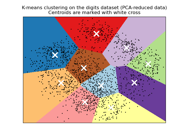
from sklearn.datasets import load_digits
digits = load_digits()
digits.data.shape

(1797, 64)

Let's see the data

• Each datapoint is a 8x8 image of a digit.

Attribute	Value
Classes	10
Samples per class	~180
Samples total	1797
Dimensionality	64
Features	int 0-15

Let's see the histogram of features (pixel colors)

_ = plt.hist(digits.data.flatten())

np.random.seed(13)  # fixing the seed to see same pictures

fig, ax = plt.subplots(2, 5, figsize=(8, 3))
idx = np.random.choice(digits.data.shape[0], 10)
labels = digits.target[idx, ...]
points = digits.data[idx, ...].reshape(-1, 8, 8)
for axi, vector, y in zip(ax.flat, points, labels):
    axi.set(xticks=[], yticks=[])
    axi.imshow(vector, interpolation='none', cmap='gray')
    axi.set_title(y)

from sklearn.model_selection import train_test_split

X_train, X_test, y_train, y_test = train_test_split(digits.data,digits.target, test_size=0.1,
                                                    random_state=0, stratify=digits.target)

plt.bar(*np.unique(y_train, return_counts=True));

plt.bar(*np.unique(y_test, return_counts=True));

Compute the mode from a distribution

Informally, the mode is the most frequent element

• We can count the frequency of each value
• Take the most frequent value

u, counts = np.unique([1,2,3,4,1,1,1,], return_counts=True)
mode = u[counts.argmax()] # will print 1 since 1 is most frequent
                          # 4 time present

Let's run our K-means on the digits

N_centers = 10 # we assume to know that there are 10 digits
centers, y_est, loss = kmeans(X_train, N_centers)

> Init with kmeans++
> Iteration 1: loss 1314.5627705627705
> Iteration 2: loss 756.8259891509574
> Iteration 3: loss 725.4550366992323
> Iteration 4: loss 716.4499767121214
> Iteration 5: loss 711.2049934919781
> Iteration 6: loss 708.236358647983
> Iteration 7: loss 705.2994723513523
> Iteration 8: loss 701.9520972059448
> Iteration 9: loss 698.6658028658622
> Iteration 10: loss 695.5144766870222
> Iteration 11: loss 693.5266489678621
> Iteration 12: loss 692.1208906914004
> Iteration 13: loss 691.3495761746228
> Iteration 14: loss 690.657571369928
> Iteration 15: loss 690.0861205462734
> Iteration 16: loss 689.7669567135049
> Iteration 17: loss 689.6771929699328
> Iteration 18: loss 689.6572694423297
> Iteration 19: loss 689.6474580308259
> Iteration 20: loss 689.6267235993998
> Iteration 21: loss 689.6114085109643

Now let's visualize the centers

fig, ax = plt.subplots(2, 5, figsize=(8, 3))
centers_img = centers.reshape(10, 8, 8)
for axi, center in zip(ax.flat, centers_img):
    axi.set(xticks=[], yticks=[])
    axi.imshow(center, interpolation='none', cmap='gray')

It looks like a smoothed version of before...

• We see that even without the labels, KMeans can find clusters whose centers are recognizable digits, with perhaps the exception of 1 and 8.
• Probably, in this case, the dataset is "easy" and distances among points have a lot of information.

• Because k-means knows nothing about the identity of the cluster, the 0–9 labels may be permuted.
  • We can fix this by matching each learned cluster label with the true labels found in them
  • In this step, we are only computing the mapping between each "color" that k-means assign to the cluster to each digit label
  • We CANNOT change the assignment to each cluster. This is meant just to map "colors" to actual digit labels.

def get_mode(X):
    values, counts = np.unique(X, return_counts=True)
    return values[counts.argmax()]

# Nx1
labels = np.zeros_like(y_est)
# 10x1
center_label = np.zeros((N_centers), dtype=np.int32)

for i in range(N_centers):
    mask = (y_est == i)
    mode_y = get_mode(y_train[mask])
    labels[mask] = mode_y
    center_label[i] = mode_y

from sklearn.metrics import accuracy_score
accuracy_score(y_train, labels)

0.7043908472479901

Accuracy of ~70% is not bad just with an unsupervised method on the "training set" though no label has been used for training

Remember: Random chance accuracy over 10 classes is 1/10 ~10%.

We also have validated our implementation of K-means

Further, There is hope this may translate to test set

# sum over axis of dimensionality of squared difference
# Nx1x64 vs 10x64 --> Nx10x64 --sum axis 2 ---> Nx10
# we match the test wrt to the center (there might be other classification methods)
L2_square = ((X_test[...,np.newaxis,:] - centers)**2).sum(axis=2)

# Nx10 -- argmin over axis --> Nx1
idx_cluster = L2_square.argmin(axis=1)

y_test_estimated = center_label[idx_cluster]

accuracy_score(y_test, y_test_estimated)

0.6722222222222223

Accuracy of ~67% is not bad just with an unsupervised method on the "test split"

Remember: Random chance accuracy over 10 classes is 1/10 ~10%

Note now things are easy because:

1. digits is an easy dataset. Which means distance in the pixel space contains useful information.
2. In the real world, unsupervised learning does not work so well.

It is OK to implement things manually in a course but remember that you can use optimized implementation via sklearn.

from sklearn.cluster import KMeans
kmeans = KMeans(n_clusters=4)
kmeans.fit(X)
y_kmeans = kmeans.predict(X)

Homework 1a: Repeat the experiments but not project the data onto a lower dimensional subspace and retain 99% of the variance. Does the classification improve? [WITHOUT sklearn, rewriting all code without looking at this; for each line of code write the matrix shape to validate your implementation]

Note: I did not try so I do not know what happens, but you can make a hypothesis. Before running it, make a hypothesis of what is going to happen following a rationale in your mind, based on what we studied so far. Then after formulating the hypothesis, do the experiments.

Tips 1: Try to retain all the features (i.e. 100% of variance) in case accuracy does not improve. In this case, you are just rotating the data and decorrelating the covariance matrix

Tips 2: If you try multiple runs, remember to FIX THE RANDOM SEED to make the experiments comparable

Homework 1b: To debug what happens, you can plot the data in 2D or 3D with PCA and show the digits ID with a color using a colormap

Homework 1c [Advanced]: To visualize the digits dataset, now use an advanced dimensionality reduction algorithm called t-SNE. Unlike PCA this method supports, multiple non-linear structures so you should see the digits more separated in 2D. For this use sklearn!

Homework 2: Repeat everything but now use sklearn.

Color Compression with K-means

# Note: this requires the ``pillow`` package to be installed
from sklearn.datasets import load_sample_image
china = load_sample_image("china.jpg")
fig, ax = plt.subplots(1, 1, figsize=(20, 15))
ax.set(xticks=[], yticks=[])
ax.imshow(china)

<matplotlib.image.AxesImage at 0x7f9b3152b370>

# Note: this requires the ``pillow`` package to be installed
from sklearn.datasets import load_sample_image
china = load_sample_image("china.jpg")
fig, ax = plt.subplots(1, 1, figsize=(20, 15))
ax.set(xticks=[], yticks=[])
ax.imshow(china)

<matplotlib.image.AxesImage at 0x7f9b40bc81c0>

• This is a (427, 640, 3) image WxHx3 where 3 is RGB but can also be seen as a 3D point cloud.
• Each pixel is a point in 3D where 3 dimensions are R, G, B

Let's normalize the data to stay in a 3D hypercube of length 1

data = china/255.0 # scale all points to 0...1
data = data.reshape(-1,3)

data = china/255.0 # scale all points to 0...1
data = data.reshape(-1,3)
data.shape

(273280, 3)

The 3D point cloud

fig = plt.figure(figsize=(15,15))
ax = fig.add_subplot(projection='3d')
data_sampled = data[::10] #1 point every 10 to go faster
ax.scatter(*data_sampled.T, marker='.', color=data_sampled)
ax.set_xlabel('R')
ax.set_ylabel('G')
_ = ax.set_zlabel('B')
ax.view_init(elev=10, azim=(0))

How many possible points are in this 3D cube?

$256^3 \approx 16$ millions

Now we quantize the colors with K-means to 16 colors

from sklearn.cluster import KMeans
kmeans = KMeans(16)
kmeans.fit(data)
y_est = kmeans.predict(data) # predict cluster center (project)
new_colors = kmeans.cluster_centers_[y_est] # backproject to the colors centers  

fig = plt.figure(figsize=(15, 15))
ax = fig.add_subplot(projection='3d')
data_sampled = new_colors[::10]  # 1 point every 10 to go faster
ax.scatter(*data_sampled.T, marker='.', color=data_sampled, s=200)
ax.set_xlabel('R')
ax.set_ylabel('G')
_ = ax.set_zlabel('B')
ax.view_init(elev=10, azim=(0))

Note

• Important: new_colors has the same shape as the original images but inside the colors get "quantized" into 16 possible colors (the k-means centers)

china_recolored = new_colors.reshape(china.shape)

fig, ax = plt.subplots(1, 2, figsize=(16, 6),
                       subplot_kw=dict(xticks=[], yticks=[]))
fig.subplots_adjust(wspace=0.05)
ax[0].imshow(china)
ax[0].set_title('Original Image (24 bit per pixel)', size=16) # 8 bit per channel, for each pixel
ax[1].imshow(china_recolored)
ax[1].set_title('16-color Image (4 bit per pixel + 24 bit per centroid)', size=16);

Bag of Visual Words: how to construct an image recogntion pipeline

Figure Credit Prof. Vedaldi - Oxford

Figure Credit Prof. Vedaldi - Oxford