Machine Learning

AI & Machine Learning - Unit 2

---

4. PCA in higher dimension, 3DMM, the curse of dimensionality

Prof. Iacopo Masi - Computer Science Department, Sapienza University of Rome

Recap previous lecture

• Principal Components Analysis (PCA)
• Eigendecomposition of a matrix
• Geometry behind PCA
• Application of PCA for:
  • Compressing the data (point cloud to line)
  • Modeling 3D Faces (3D Morphable Model 3DMM)
  • Rotating the data

Today's lecture

PCA with SVD

PCA in a high dimensional space

Application: Eigenfaces

Eigendecomposition of Matrices

$$ \mathbf{W} = \begin{bmatrix} 1 & 1 \\ -1 & 2 \end{bmatrix}, $$

be the matrix where the columns are the eigenvectors of the matrix $\mathbf{A}$. Let

$$ \boldsymbol{\Sigma} = \begin{bmatrix} 1 & 0 \\ 0 & 4 \end{bmatrix}, $$

be the matrix with the associated eigenvalues on the diagonal. Then the definition of eigenvalues and eigenvectors tells us that

$$ \mathbf{A}\mathbf{W} =\mathbf{W} \boldsymbol{\Sigma} . $$

If the matrix $\mathbf{W}$ is invertible, we may multiply both sides by $W^{-1}$ on the right, we see that we may write

$$\mathbf{A} = \mathbf{W} \boldsymbol{\Sigma} \mathbf{W}^{-1}.$$

Operations on Eigendecompositions

One nice thing about eigendecompositions is that we can write many operations we usually encounter cleanly in terms of the eigendecomposition. As a first example, consider:

$$ \mathbf{A}^n = \overbrace{\mathbf{A}\cdots \mathbf{A}}^{\text{$n$ times}} = \overbrace{(\mathbf{W}\boldsymbol{\Sigma} \mathbf{W}^{-1})\cdots(\mathbf{W}\boldsymbol{\Sigma} \mathbf{W}^{-1})}^{\text{$n$ times}} = \mathbf{W}\overbrace{\boldsymbol{\Sigma}\cdots\boldsymbol{\Sigma}}^{\text{$n$ times}}\mathbf{W}^{-1} = \mathbf{W}\boldsymbol{\Sigma}^n \mathbf{W}^{-1}. $$

This tells us that for any positive power of a matrix, the eigendecomposition is obtained by just raising the eigenvalues to the same power. The same can be shown for negative powers, so if we want to invert a matrix we need only consider

$$ \mathbf{A}^{-1} = \mathbf{W}\boldsymbol{\Sigma}^{-1} \mathbf{W}^{-1}, $$

or in other words, just invert each eigenvalue.

Eigendecompositions of Symmetric Matrices

• Hessian
• Covariance Matrices*
• PCA*
• Kernels etc

Eigendecompositions and Singular Value Decomposition

Method	$\mathbf{A}$	Decomposition
SVD	any	$\mathbf{A}=\mathbf{U}\mathbf{\Sigma}\mathbf{V}^T$
Eigen	square	$\mathbf{A}=\mathbf{U}\mathbf{\Sigma}\mathbf{U}^{-1}$
Eigen	square/sym	as above but $\mathbf{U}\mathbf{U}^T=\mathbf{I}$

Decomposition as a Geometric Pipeline

$$\mathbf{A}\mathbf{x} = \underbrace{(\mathbf{U} \underbrace{(\mathbf{\Sigma}\underbrace{(\mathbf{U}^{-1}\mathbf{x})}_{\text{1st step/rotate}})}_{\text{2nd step/scale and flip}})}_{\text{3rd step/rotate}}$$

Method	Step 1	Step 2	Step 3
geometry	rotate	scale axis	rotate
SVD	$\mathbf{V}^T$	$\mathbf{\Sigma}$	$\mathbf{U}$
geometry	rotate	scale axis	rotate back
Eig	$\mathbf{U}^{-1}$	$\mathbf{\Sigma}$	$\mathbf{U}$

Decomposition as a Geometric Pipeline

Geometry of SVD

Source: wikipedia

Principal Component Analysis (PCA)

PCA works in unsupervised learning settings

\begin{equation} \underbrace{\{\mathbf{x}_i\}_{i=1}^N}_{\text{known}} \sim \underbrace{\mathcal{D}}_{\text{unknown}} \end{equation}

Assumptions

• $\mathbf{x}_i \in \mathbb{R}^D$
• $N \geq D$ (number of points higher than number of features; or else, more points than dimensions)

Objective: find a transformation (subspace) for compressing the data

Find the projection that maximizes the spread of the data

• Find $\mathbf{u}\in \mathbb{R}^k$ $\left\|\mathbf{u}\right\|_2=1$ for which you can project the data $\mathbf{x}^{\prime}=\mathbb{P}_{\mathbf{u}}\mathbf{x}$

$$ \mathbb{P}_{\mathbf{u}}\mathbf{x} = (\mathbf{x}^T\mathbf{u})\mathbf{u}$$

• We have to maximize the variance once projected.
• Which means projecting x with u large (U):
• We can measure the size of the projection with the $\ell_2$ norm.

$$\arg\max_{\mathbf{u}} \frac{1}{N}\sum_i^N \left\| (\mathbf{x}_i^T\mathbf{u})\mathbf{u}\right\|_2^2$$

Full recipe

$$ \mathbf{X}^{\prime} \leftarrow \frac{\mathbf{X} - \mathbf{\mu}}{\mathbf{\sigma}} $$$$\underbrace{\mathbf{x}^{T\prime}_p}_{\text{rec}} = \underbrace{\underbrace{\mathbf{U}_{|k}}_{k \mapsto D}\quad\underbrace{\underbrace{\mathbf{U}_{|k}^T}_{D \mapsto k}\quad\underbrace{\mathbf{x}^{T\prime}}_{\text{orig}}}_{projection}}_{reconstruction}$$$$ \mathbf{x}_p\leftarrow\left(\mathbf{x}^{T\prime}_p{\mathbf{\sigma}}\right)+\mathbf{\mu}$$

Can be used for compressing and reconstructing the data using U up to k components: $$\underbrace{\mathbf{x}^T}_{\text{prj}} = \underbrace{\underbrace{\mathbf{U}_{|k}}_{k \mapsto D}\quad\underbrace{\underbrace{\mathbf{U}_{|k}^T}_{D \mapsto k}\quad\underbrace{\mathbf{x}^T}_{\text{orig}}}_{projection}}_{reconstruction}$$

Alternative interpretation: Find orthogonal projection that minimizes reconstruction error

$\def\mbf#1{\mathbf{#1}}$

• Find an orthogonal matrix $\mbf{U}\in \mathbb{R}^{D\times k}$ for which:

$$\arg\min_{\mbf{U}} \left\| \mbf{X} - \mbf{U}\mbf{U}^T\mbf{X}\right\|_2^2 \\ \text{subject to} \quad \mbf{U}^T\mbf{U} = \mbf{I_k} $$

• Both interpretations lead to the same results:
  • To compute $\mbf{U}$ you have to compute Eigendecomposition of covariance matrix $\frac{1}{N}\mbf{X}\mbf{X}^T$

What happens if input dimensionality is large?

• $\mbf{X} \in \mathbb{R}^{D\times N}$ then $\mathbb{Cov} = \frac{1}{N}\mbf{X}\mbf{X}^T$ is a big matrix.
• $D \gg N$

What is the shape of $\mathbb{Cov}$?

• $\mathbb{Cov} \in \mathbb{R}^{D\times D}$.
• Eigendecomposition complexity $\mathcal{O}(D^3)$ so, in our case, if $D$ is large we have a computational problem.

What happens in high dimensions?

• Are we supposed to think about the world in a 3-dimensional space?
• Our brain can think in a 3-dimensional world.
• Maybe with relativity theory, we arrive at a 4-D space if we also consider time.
• So why do we need higher dimensions?

High Dimensional Space

• Visualizing one-hundred-dimensional space is incredibly difficult for humans.
• Most of the time the representation for an input datum is a vector in high dimensional space.

• You can think of an image $\mathbf{I}\in \mathbb{R}^{WxH}$ as a point/vector in high dimension.
• For an image $128\times 128$ now our $D$ dimension is very high. $D=128^2=(2^7)^2=2^{14}\approx16K$

• Let's double the image $128 \mapsto 256$

• For an image $256\times 256$ now our $D$ dimension is very high. $D=256^2=(2^8)^2=2^{16}\approx65K$
• Doubling a side increases the dimension four times, due to the two-dimensional nature of images.

• So you can consider an image as a $65K$-dimensional vector!

Let's practice with 2D real data

We will pull a 2D real dataset made of images in the wild using sklearn

from sklearn.datasets import fetch_lfw_people
faces = fetch_lfw_people(min_faces_per_person=60)
print(faces.target_names)
print(faces.images.shape)

['Ariel Sharon' 'Colin Powell' 'Donald Rumsfeld' 'George W Bush'
 'Gerhard Schroeder' 'Hugo Chavez' 'Junichiro Koizumi' 'Tony Blair']
(1348, 62, 47)

faces.images[0,...].shape

(62, 47)

Best Practice: Always look at the data before you start working!

• Do not do simple summary statistics on the dataset
• Always look at large random samples of the dataset
• The data may contain noise that you want to be aware of!
• Do not take for granted that the data and the labels are noise-free
• You could try to plot the data to a lower dimension also (i.e. with PCA)

In total we have (1348, 62, 47) so 1348 images of dimension 62x47 = 2914.

# Plot the faces
N_ax, N_img = 10, 10 #10 rows with 10 images per row
fig, ax = plt.subplots(N_ax, N_img,figsize=(10,10),
                       subplot_kw={'xticks':[], 'yticks':[]},
                       gridspec_kw=dict(hspace=0.1, wspace=0.1))
for i in range(N_ax):
    ax[i,0].set_ylabel(f'Faces {i}')
    for j in range(N_img):
        ax[i,j].imshow(faces.data[i*N_img+j].reshape(62, 47), cmap='gray')

For example, what is this?

plt.imshow(faces.data[9*N_img].reshape(62, 47), cmap='gray')

<matplotlib.image.AxesImage at 0x7fd499e50ca0>

• Looks like a misalignment error!
• This can create noise in PCA estimation

2D images are high-dimensional vectors

• We said faces are vectors that live in a $\mathbb{[0,255]}^{2914}$, if you flatten the dimensions
• Now how many images can you draw in this space, assuming the grayscale values are $[0,\ldots,255]$?

$$256^{H\times W}=256^{2914} \approx 10^{7018}$$

Long Story Short

• The $WxH$ where the faces live defined a HUGE space
• The face samples from this space occupy a very tiny portion of the space
• That is, the space is very sparse given its huge "possible" volume
• Note: the same holds for natural images (not just for faces).

Let's random sample uniformly the space in 2914 dimensions

• This is because there is a difference between:
  1. The space where the data lives (what you see with the image)
  2. The "real" unseen space where the data may be embedded.

# Sampling
samples = np.random.uniform(0, 255, (100, 62, 47)).astype(np.uint8)
# uniformly sample 100 points in 62x47 space.

# Plot the faces
N_ax, N_img = 10, 10  # 10 rows with 10 images per row
fig, ax = plt.subplots(N_ax, N_img, figsize=(10, 10),
                       subplot_kw={'xticks': [], 'yticks': []},
                       gridspec_kw=dict(hspace=0.1, wspace=0.1))
for i in range(N_ax):
    ax[i, 0].set_ylabel(f'Samples {i}')
    for j in range(N_img):
        ax[i, j].imshow(samples[i*N_img+j].reshape(62, 47), cmap='gray')

# Sampling
samples = np.random.uniform(0, 255, (100, 62, 47)).astype(np.uint8)
# uniformly sample 100 points in 62x47 space.

# Plot the faces
N_ax, N_img = 10, 10  # 10 rows with 10 images per row
fig, ax = plt.subplots(N_ax, N_img, figsize=(10, 10),
                       subplot_kw={'xticks': [], 'yticks': []},
                       gridspec_kw=dict(hspace=0.1, wspace=0.1))
for i in range(N_ax):
    ax[i, 0].set_ylabel(f'Samples {i}')
    for j in range(N_img):
        ax[i, j].imshow(samples[i*N_img+j].reshape(62, 47), cmap='gray')

The probability of hitting a face is very small!

The phenomenon is also known as...

The curse of dimensionality

• Fixing the samples you have in a training set, then
• as the dimensionality grows $\rightarrow$ fewer examples in each region of the feature space

The curse of dimensionality

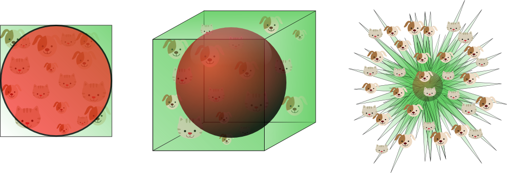
• The number of training samples must grow exponentially with dimensionality if we want to maintain the same "density"

• This also means [informally] that if you increase the input dimension, the number of your training samples should grow exponentially to have the same performance and avoid "overfitting".

• More on overfitting later but let's say for now that overfitting = ML method not working well

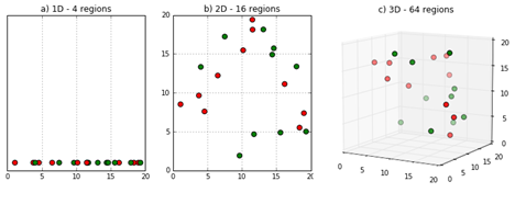
Figure Credit DeepAI

Ambient space

_=plt.imshow(faces.data[0*N_img].reshape(62, 47), cmap='gray')

Embedded space

$$\underbrace{\mathbf{I}}_{\text{what you see}} = \mathcal{G}(\text{id}, \text{pose}, \text{age}, \text{etnicity}, \text{illumination})$$

Faces may be "living" in a lower embedded space defined by:

1. Identity
2. Pose
3. Age
4. Ethnicity etc.

Stranger things happen in higher dimensions

• As D increases, the volume of the hypersphere goes to zero while the hyper-cube remains constant.
• Training samples may be located at the corners of the hypercube.

Credit Vincent Spruyt

Distances in high-dimensional space

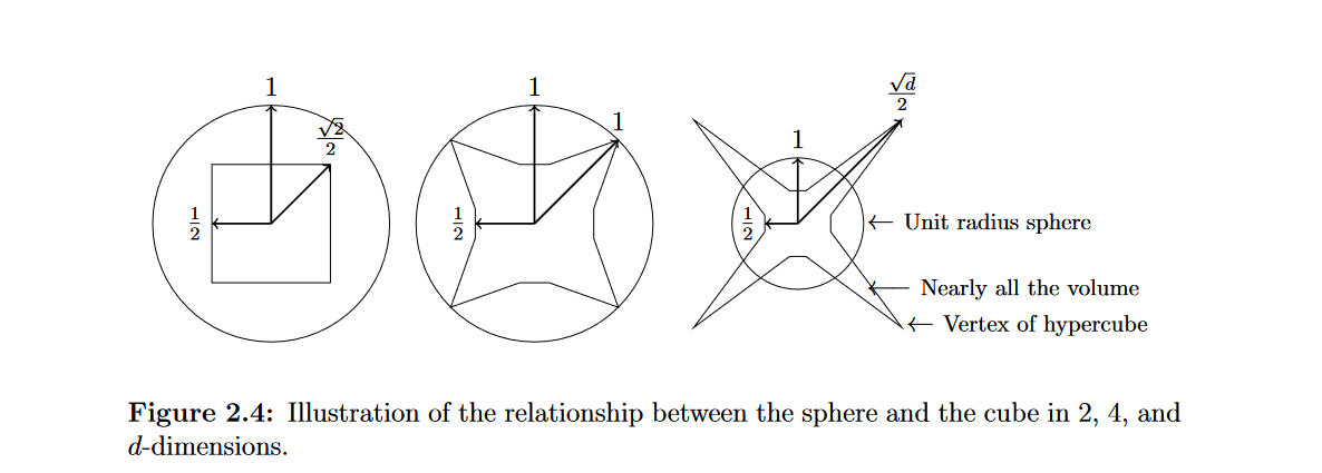
Distances in high dimensions follow a pattern:

• Distance of points sampled on the unit sphere goes to zero as D increases.
• Euclidean distance of points goes to $4\sqrt{D}$.
• The variance of distances between two random points keeps shrinking as D increases.

Figure Credit from this paper

See this chapter for more explanations

Dimensionality in ML: some reference numbers

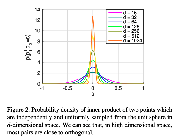
• D ≈ 20 is considered “low dimensional,”
• D ≈ 1,000 is “medium dimensional”
• D ≈ 100,000 is “high dimensional”.

Eigenfaces (i.e. PCA applied to 2D images)

from sklearn.decomposition import PCA 

pca = PCA(n_components=150) # retain 150 components
print(faces.data.shape) #NxD N=1348 samples in ~3K-D space
pca.fit(faces.data)

(1348, 2914)

PCA(n_components=150)

fig, axes = plt.subplots(3, 8, figsize=(9, 4),
                         subplot_kw={'xticks':[], 'yticks':[]},
                         gridspec_kw=dict(hspace=0.1, wspace=0.1))
for i, ax in enumerate(axes.flat):
    if i == 0:
        ax.imshow(pca.mean_.reshape(62, 47), cmap='bone') #  plot mean
    else:
        ax.imshow(pca.components_[i].reshape(62, 47), cmap='gray') # plots components

plt.figure(figsize=(20,10))
plt.plot(np.cumsum(pca.explained_variance_ratio_))
plt.xlabel('number of components')
plt.ylabel('cumulative explained variance');
_ = plt.ylim([0,1])

Subspaces in decreasing order of variance

$$ (\lambda_1,\mathbf{u}_1),\ldots,(\lambda_d,\mathbf{u}_d) = \text{eig}(\frac{1}{N}\mathbf{X}^T\mathbf{X}) $$

Note: *numpy is not guaranteed to return it ordered so you have to sort*

How do we choose the subspace where to cut the dimension?

• From $D$-dimensional to $k$-dimension
• Given the spectrum $$\mathbf{\Sigma} = \text{diag}(\lambda_1,...,\lambda_d)$$ we can remove the dimension considering the spectrum "energy" and retain e.g. 95% of the variance in data.

That is, Keep k components until:

$$\frac{\sum_i^k \lambda_i}{\sum_i^d \lambda_i} \leq 95\%$$

Data compression

• The first 150 components explain more than 90% of the data!
• From $2914$ space to $150$ space with no loss of information?
• Let's project back to the input space and see.

plt.rcParams['axes.grid'] = False
from mpl_toolkits.axes_grid1.axes_divider import make_axes_locatable
# Project back to the input
# Project back to the input
projected = pca.transform(faces.data) # project with P = U_t*X_t
unprojected = pca.inverse_transform(projected) # unproject with U*P = U(U_t*X_t)
# Now plot
fig, ax = plt.subplots(3, 10, figsize=(35, 10),
                       subplot_kw={'xticks': [], 'yticks': []},
                       gridspec_kw=dict(hspace=0.1, wspace=0.1))

# it is important to get the max value of the error so that
# we plot heatmap error with the SAME SCALE!
errors_img = [(unprojected[i]-faces.data[i])**2 for i in range(10)]
max_val = max([err.max() for err in errors_img])

for i in range(10):
    ax[0, i].imshow(faces.data[i].reshape(62, 47), cmap='gray')
    ax[1, i].imshow(unprojected[i].reshape(62, 47), cmap='gray')
    erri = ax[2, i].imshow((errors_img[i]).reshape(
        62, 47), cmap='jet', extent=[0, max_val]*2)
    if i == 9:
        divider = make_axes_locatable(ax[2, i])
        cax = divider.append_axes("right", size="5%", pad=0.005)
        plt.colorbar(erri, cax=cax)

ax[0, 0].set_ylabel('full-dim\ninput')
ax[1, 0].set_ylabel('150-dim\nreconstruction')
_ = ax[2, 0].set_ylabel('L2 rec. err')

plt.rcParams['axes.grid'] = False
from mpl_toolkits.axes_grid1.axes_divider import make_axes_locatable
# Project back to the input
# Project back to the input
projected = pca.transform(faces.data) # project with P = U_t*X_t
unprojected = pca.inverse_transform(projected) # unproject with U*P = U(U_t*X_t)
# Now plot
fig, ax = plt.subplots(3, 10, figsize=(35, 10),
                       subplot_kw={'xticks': [], 'yticks': []},
                       gridspec_kw=dict(hspace=0.1, wspace=0.1))

# it is important to get the max value of the error so that
# we plot heatmap error with the SAME SCALE!
errors_img = [(unprojected[i]-faces.data[i])**2 for i in range(10)]
max_val = max([err.max() for err in errors_img])

for i in range(10):
    ax[0, i].imshow(faces.data[i].reshape(62, 47), cmap='gray')
    ax[1, i].imshow(unprojected[i].reshape(62, 47), cmap='gray')
    erri = ax[2, i].imshow((errors_img[i]).reshape(
        62, 47), cmap='jet', extent=[0, max_val]*2)
    if i == 9:
        divider = make_axes_locatable(ax[2, i])
        cax = divider.append_axes("right", size="5%", pad=0.005)
        plt.colorbar(erri, cax=cax)

ax[0, 0].set_ylabel('full-dim\ninput')
ax[1, 0].set_ylabel('150-dim\nreconstruction')
_ = ax[2, 0].set_ylabel('L2 rec. err')

Let's try with only 3 Components!

from mpl_toolkits.axes_grid1.axes_divider import make_axes_locatable

############### Fitting with 3 components ######
pca = PCA(n_components=3) # retain 3 components
pca.fit(faces.data)
#############################################
##### Plot
# Project back to the input
projected = pca.transform(faces.data) # project with P = U_t*X_t
unprojected = pca.inverse_transform(projected) # unproject with U*P = U(U_t*X_t)
# Now plot
fig, ax = plt.subplots(3, 10, figsize=(15, 4.5),
                       subplot_kw={'xticks': [], 'yticks': []},
                       gridspec_kw=dict(hspace=0.1, wspace=0.1))

# it is important to get the max value of the error so that
# we plot heatmap error with the SAME SCALE!
errors_img = [(unprojected[i]-faces.data[i])**2 for i in range(10)]
max_val = max([err.max() for err in errors_img])

for i in range(10):
    ax[0, i].imshow(faces.data[i].reshape(62, 47), cmap='gray')
    ax[1, i].imshow(unprojected[i].reshape(62, 47), cmap='gray')
    erri = ax[2, i].imshow((errors_img[i]).reshape(
        62, 47), cmap='jet', extent=[0, max_val]*2)
    if i == 9:
        divider = make_axes_locatable(ax[2, i])
        cax = divider.append_axes("right", size="5%", pad=0.005)
        plt.colorbar(erri, cax=cax)

ax[0, 0].set_ylabel('full-dim\ninput')
ax[1, 0].set_ylabel('3-dim\nreconstruction')
_ = ax[2, 0].set_ylabel('L2 rec. err')

# Nx3
fig = plt.figure(figsize=(5,5))
ax = fig.add_subplot(projection='3d')
_ = ax.scatter(*projected.T, c=faces.target, marker='.', cmap='jet')

Color maps to Identity

Looks like not a great projection for separating the identity!

In the end makes sense since PCA is an unsupervised method.

Another example for PCA on color RGB images on CIFAR-10

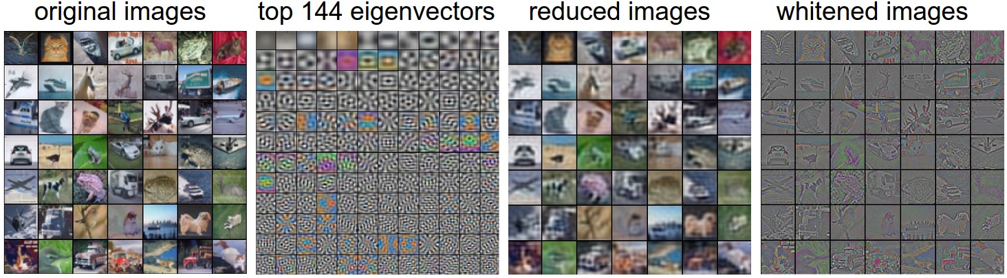
[Taken from cs231n.github.io/neural-networks-2](https://cs231n.github.io/neural-networks-2/)

Now I will show you some data and then you need to tell me if using

PCA is a good way to separate the color of the data

plt.figure(figsize=(10,10))
np.random.seed(0)
N_samples = 50
# samples points for class 1
X_1 = np.random.uniform(50, 200, N_samples)
X_1 = np.vstack((X_1, (1,)*N_samples))
# samples points for class 2
X_2 = np.random.uniform(50, 200, N_samples)
X_2 = np.vstack((X_2, (20,)*N_samples))
X = np.concatenate((X_1, X_2))
# data
X = np.concatenate((X_1, X_2), axis=1)
# labels
labels = X[1, ...]
# Plot also the training points
plt.scatter(
    x=X[0, ...],
    y=X[1, ...],
    c=labels,
    cmap='jet',
)
# Code below wants Nx2
X = X.T
_ = plt.axis('equal')

Why compression

This example is just used for illustrative purposes since Machine Learning is much related to Information Theory.

How to apply PCA

Usage of PCA

• Inductive (estimate basis on training set); apply on test set - Most common
• Transductive (get all the points at test time; estimate and project) - Assumes you have all the points at test time

Inductive Settings

Most of the methods covered in this course are "Inductive" (as opposed to transductive).

• Induction works well for supervised methods but can also be applied to unsupervised methods.
• [Training] Estimate $\mbf{U}$ on a training set (and also mean $\mu$ and std $\sigma$)
• [Test Time] Given a new point $\mbf{x}^{\prime}$ at test-time, apply PCA, that is project $\mbf{x}^{\prime}$ with $\mbf{U}, \mu, \sigma$

On the side: Transductive Settings

Vapnik'98 - Learning by Transduction